Unit 2: CPU Scheduling

1. Introduction to CPU Scheduling

CPU scheduling is the basis of multiprogrammed operating systems. By switching the CPU among processes, the operating system can make the computer more productive.

1.1 Basic Concepts

• CPU-I/O Burst Cycle: Process execution consists of a cycle of CPU execution and I/O wait. Processes alternate between these two states.
  • CPU-bound processes: Spend more time doing computations (long CPU bursts).
  • I/O-bound processes: Spend more time waiting for I/O (short CPU bursts).
• The Goal: To maximize CPU utilization by keeping the CPU busy at all times. When one process waits for I/O, the scheduler selects another process from the ready queue to run.

1.2 CPU Scheduler

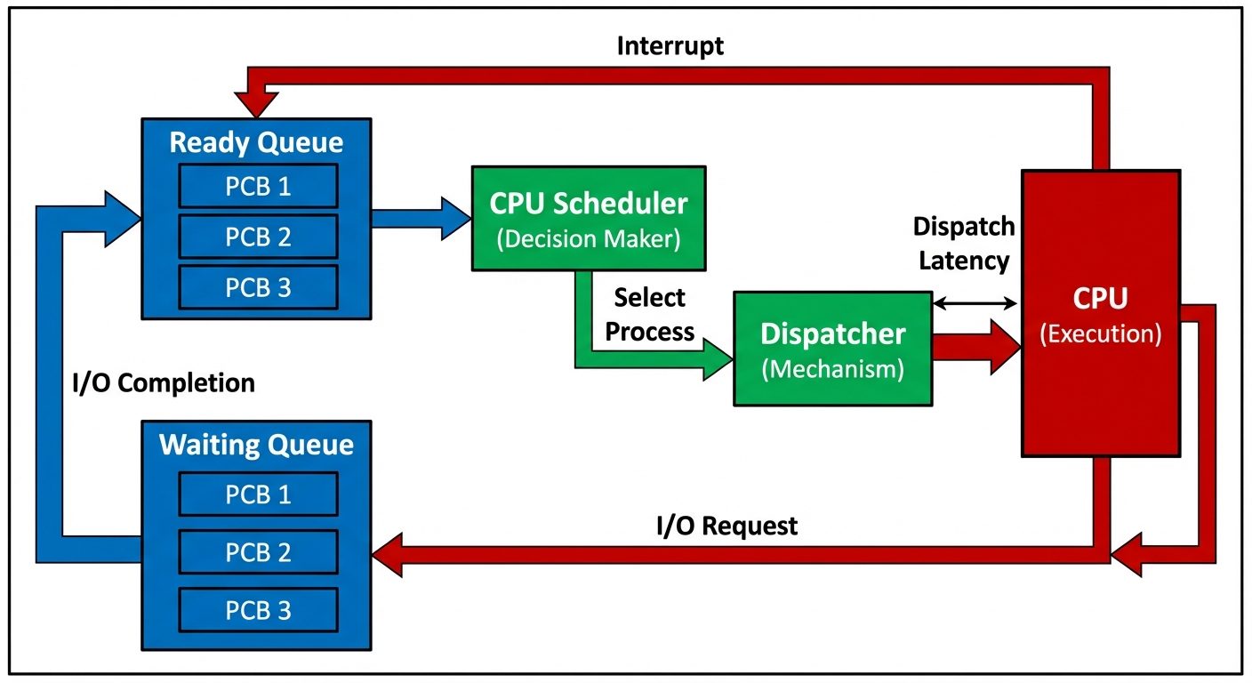
The CPU Scheduler (Short-Term Scheduler) selects a process from the processes in memory that are ready to execute and allocates the CPU to that process.

Types of Scheduling Decisions

Scheduling decisions may take place when a process:

1. Switches from running to waiting state (e.g., I/O request).
2. Switches from running to ready state (e.g., interrupt occurs).
3. Switches from waiting to ready (e.g., I/O completion).
4. Terminates.

Preemptive vs. Non-Preemptive Scheduling

• Non-Preemptive (Cooperative): Once the CPU has been allocated to a process, the process keeps the CPU until it releases it either by terminating or switching to the waiting state (Conditions 1 and 4).
• Preemptive: The CPU can be taken away from a currently running process before it finishes its burst (Conditions 2 and 3). This requires hardware support (timers) and can lead to race conditions.

1.3 The Dispatcher

The dispatcher is the module that gives control of the CPU to the process selected by the short-term scheduler. It is different from the scheduler; the scheduler makes the decision, the dispatcher performs the action.

Functions of the Dispatcher:

• Context Switching: Saving the state of the current process and loading the state of the new process.
• Switching to User Mode.
• Jumping to the proper location in the user program to restart that program.

Dispatch Latency: The time it takes for the dispatcher to stop one process and start another running. This must be minimized.

2. Scheduling Criteria

To compare CPU scheduling algorithms, the following characteristics are used:

Maximizing Performance

• CPU Utilization: Keep the CPU as busy as possible (range 0% to 100%).
• Throughput: Number of processes that complete their execution per time unit.

Minimizing Inefficiency

• Turnaround Time: The interval from the time of submission of a process to the time of completion.
  • Formula:
• Waiting Time: The sum of the periods spent waiting in the ready queue.
  • Formula:
• Response Time: The time from the submission of a request until the first response is produced (critical for interactive systems).

3. Scheduling Algorithms

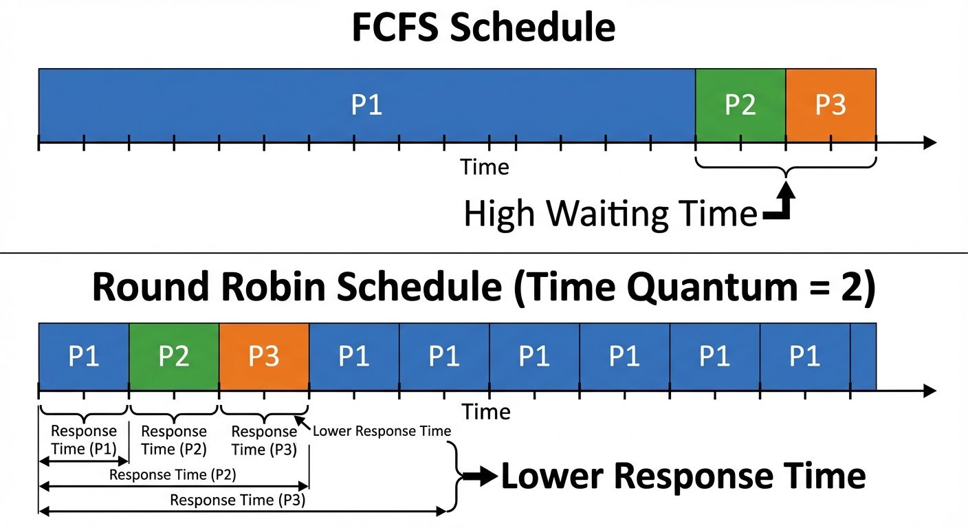
3.1 First-Come, First-Served (FCFS)

• Type: Non-Preemptive.
• Logic: The process that requests the CPU first is allocated the CPU first. Implemented using a FIFO queue.
• Pros: Simple to write and understand.
• Cons:
  • High average waiting time.
  • Convoy Effect: Short processes stuck waiting behind a long CPU-bound process.

3.2 Shortest Job First (SJF)

• Type: Can be Non-Preemptive or Preemptive (Shortest Remaining Time First - SRTF).
• Logic: Associate with each process the length of its next CPU burst. Use these lengths to schedule the process with the shortest time.
• Pros: Gives the minimum average waiting time for a given set of processes (Optimal).
• Cons:
  • Difficult to implement because the length of the next CPU burst is not known in advance (requires exponential averaging to predict).
  • Possible starvation for long processes.

3.3 Priority Scheduling

• Type: Preemptive or Non-Preemptive.
• Logic: A priority number (integer) is associated with each process. The CPU is allocated to the process with the highest priority (convention varies: sometimes 0 is high, sometimes low).
• Problem - Starvation (Indefinite Blocking): Low priority processes may never execute.
• Solution - Aging: Gradually increase the priority of processes that wait in the system for a long time.

3.4 Round Robin (RR)

• Type: Preemptive.
• Logic: Designed for time-sharing systems. Similar to FCFS, but preemption is added to switch between processes.
• Time Quantum (q): A small unit of time (e.g., 10-100 ms).
  • If burst < q: Process releases CPU voluntarily.
  • If burst > q: Timer interrupt goes off, context switch happens, process put at tail of ready queue.
• Performance: Depends heavily on the size of the time quantum.
  • Large q: Becomes FCFS.
  • Small q: High context switch overhead.

4. Advanced Queueing Algorithms

4.1 Multilevel Queue Scheduling

• Concept: Partitions the ready queue into several separate queues (e.g., foreground/interactive and background/batch).
• Constraint: Processes are permanently assigned to one queue based on memory size, priority, or process type.
• Scheduling: Each queue has its own scheduling algorithm (e.g., RR for foreground, FCFS for background). There must be scheduling between the queues (usually Fixed-priority preemptive).

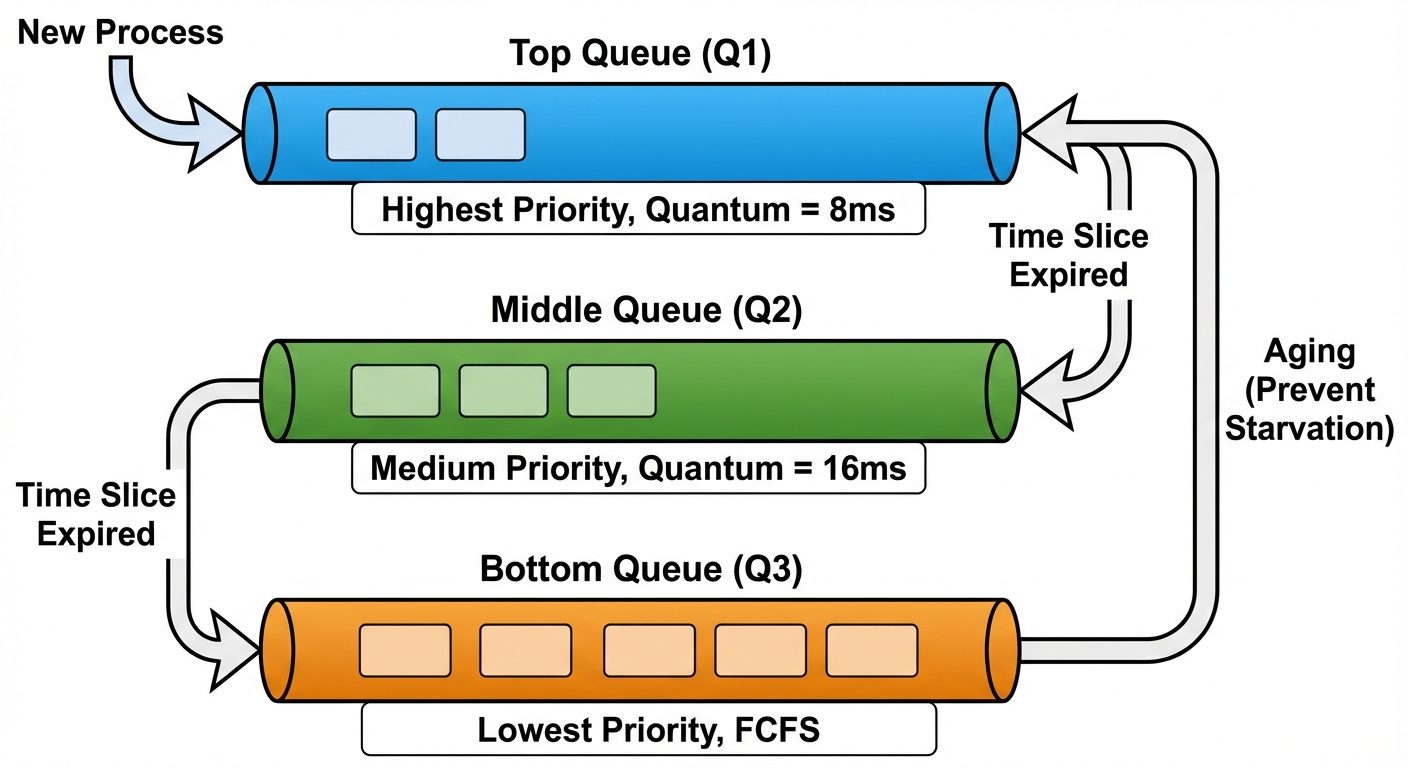
4.2 Multilevel Feedback Queue (MLFQ)

• Difference: Allows a process to move between queues.
• Logic: Separate processes according to the characteristics of their CPU bursts. If a process uses too much CPU time, it is moved to a lower-priority queue. I/O-bound and interactive processes stay in the higher-priority queues.
• Parameters:
  1. Number of queues.
  2. Scheduling algorithm for each queue.
  3. Method to determine when to upgrade a process (Aging).
  4. Method to determine when to demote a process.

5. Thread Scheduling

On operating systems that support threads, it is kernel-level threads—not processes—that are being scheduled.

5.1 Scope of Contention

1. Process-Contention Scope (PCS): On systems implementing many-to-one or many-to-many models, the thread library schedules user-level threads to run on an available LWP (Lightweight Process). This happens within the process.
2. System-Contention Scope (SCS): The kernel decides which kernel-level thread to schedule onto a CPU. This competes with all threads in the system.

6. Multiprocessor Scheduling

When multiple CPUs are available, load sharing becomes possible, but scheduling becomes more complex.

6.1 Approaches

• Asymmetric Multiprocessing: One "master" server handles all scheduling decisions, I/O processing, and system activities. The other processors execute only user code. Simple, but the master is a bottleneck.
• Symmetric Multiprocessing (SMP): Each processor is self-scheduling. All processors may be in a common ready queue, or each may have its own private queue of ready processes. Most modern OSs (Windows, Linux, macOS) use SMP.

6.2 Load Balancing (in SMP)

Necessary to keep the workload evenly distributed across all processors.

• Push Migration: A specific task checks load periodically and pushes processes from overloaded CPUs to idle ones.
• Pull Migration: An idle processor pulls a waiting task from a busy processor.

6.3 Processor Affinity

Processes have an affinity for the processor on which they are currently running (due to cache memory population).

• Soft Affinity: OS attempts to keep the process on the same CPU but doesn't guarantee it.
• Hard Affinity: System calls allow specifying a subset of processors on which a process may run.

7. Real-Time Scheduling

Real-time systems are defined by their ability to complete tasks within a specific time constraint (deadline).

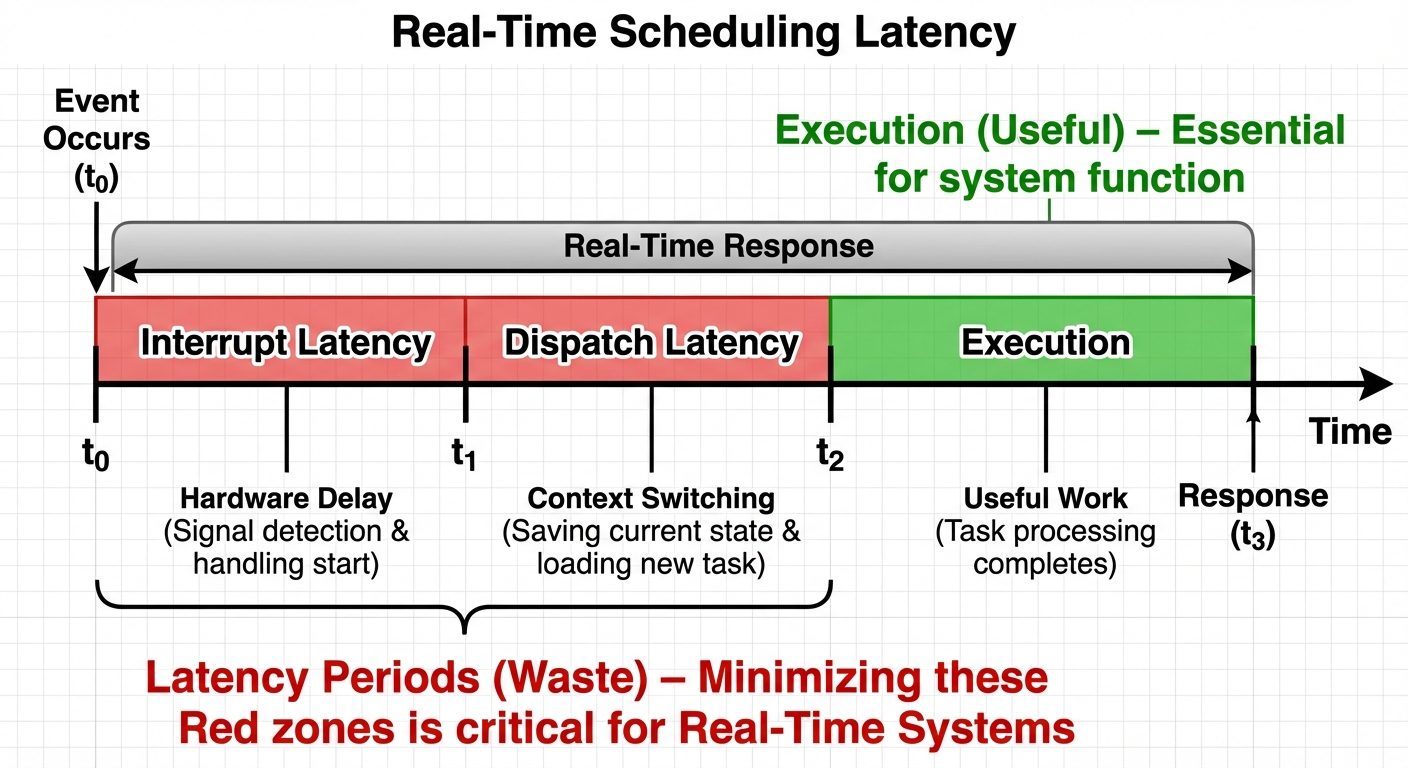
7.1 Types of Latency

• Interrupt Latency: Time from arrival of interrupt to start of the interrupt service routine.
• Dispatch Latency: Time for scheduler to take current process off CPU and switch to another.

7.2 Categories

1. Soft Real-Time: Critical real-time processes get preference over non-critical processes, but no guarantee as to when they will be scheduled.
2. Hard Real-Time: A task must be serviced by its deadline; service after the deadline is the same as no service at all.

7.3 Algorithms

• Rate Monotonic Scheduling: A static priority policy using preemption. Shorter periods = Higher priority.
• Earliest Deadline First (EDF): A dynamic priority policy. The closer the deadline, the higher the priority.