Unit 2: Pandas for Data Handling

Pandas is an open-source Python library providing high-performance, easy-to-use data structures and data analysis tools. It is built on top of NumPy and is essential for data cleaning, manipulation, and analysis in Machine Learning.

1. Series and DataFrame

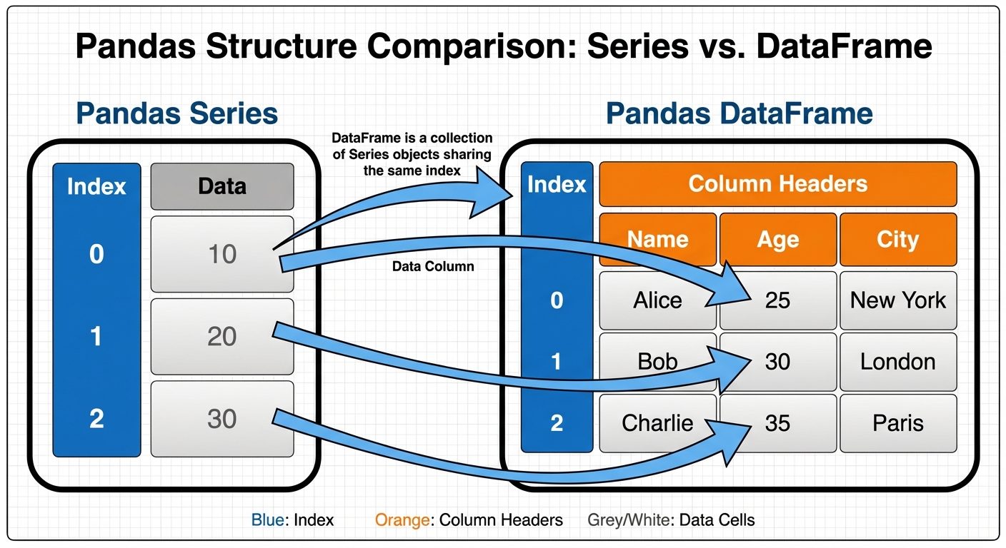
Pandas deals primarily with two data structures: Series (1-dimensional) and DataFrame (2-dimensional).

1.1 Pandas Series

A Series is a one-dimensional labeled array capable of holding data of any type (integer, string, float, python objects, etc.). The axis labels are collectively called the index.

Syntax:

import pandas as pd
s = pd.Series(data, index=index)

Example:

import pandas as pd
import numpy as np

# Creating a Series from a list
data = [10, 20, 30, 40]
labels = ['a', 'b', 'c', 'd']
series = pd.Series(data, index=labels)

print(series)
# Output:
# a    10
# b    20
# c    30
# d    40
# dtype: int64

1.2 Pandas DataFrame

A DataFrame is a two-dimensional data structure, i.e., data is aligned in a tabular fashion in rows and columns. It is mutable, size-mutable, and can handle heterogeneous data types.

Key Features:

• Potentially columns are of different types.
• Size – Mutable.
• Labeled axes (rows and columns).
• Can perform arithmetic operations on rows and columns.

Example:

# Creating a DataFrame from a Dictionary
data = {
    'Name': ['Alice', 'Bob', 'Charlie'],
    'Age': [25, 30, 35],
    'City': ['New York', 'Paris', 'London']
}

df = pd.DataFrame(data)
print(df)

2. Reading and Writing CSV Files

CSV (Comma Separated Values) is the most common file format for storing data.

2.1 Reading CSV

The read_csv() function is used to load a CSV file into a DataFrame.

# Basic reading
df = pd.read_csv('data.csv')

# Reading with specific requirements
df = pd.read_csv('data.csv', 
                 index_col=0,       # Use first column as index
                 header=0,          # Row number to use as column names
                 usecols=['Name', 'Age']) # Load specific columns

2.2 Writing CSV

The to_csv() function writes a DataFrame to a CSV file.

# Write to CSV
df.to_csv('output.csv', index=False) # index=False prevents writing row numbers

3. Inspecting Datasets

Before analyzing data, it is crucial to understand its structure and content.

4. Selecting and Filtering Data

Pandas provides specific accessors, loc and iloc, for efficient data selection.

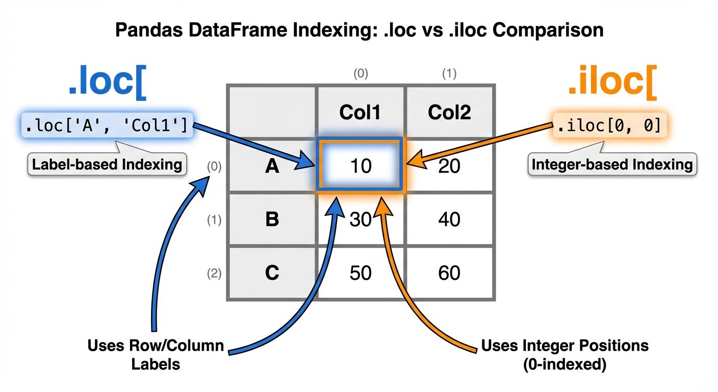
4.1 Selection: loc vs iloc

• loc (Label-based): Selects data based on the names of rows and columns.
• iloc (Integer-based): Selects data based on the integer position (index) of rows and columns (0-based).

Example:

# Select the row with index label 'a' and column 'Age'
val = df.loc['a', 'Age'] 

# Select the first row (position 0) and the second column (position 1)
val = df.iloc[0, 1]

# Slicing
subset_loc = df.loc[:, 'Name':'Age'] # All rows, columns from Name to Age (inclusive)
subset_iloc = df.iloc[0:5, 0:2]      # First 5 rows, first 2 columns (exclusive of end)

4.2 Filtering (Boolean Indexing)

Filtering allows you to select rows that satisfy a specific condition.

# Filter rows where Age is greater than 30
adults = df[df['Age'] > 30]

# Multiple conditions (Use & for AND, | for OR)
# Note: Parentheses are mandatory around conditions
target_group = df[(df['Age'] > 25) & (df['City'] == 'London')]

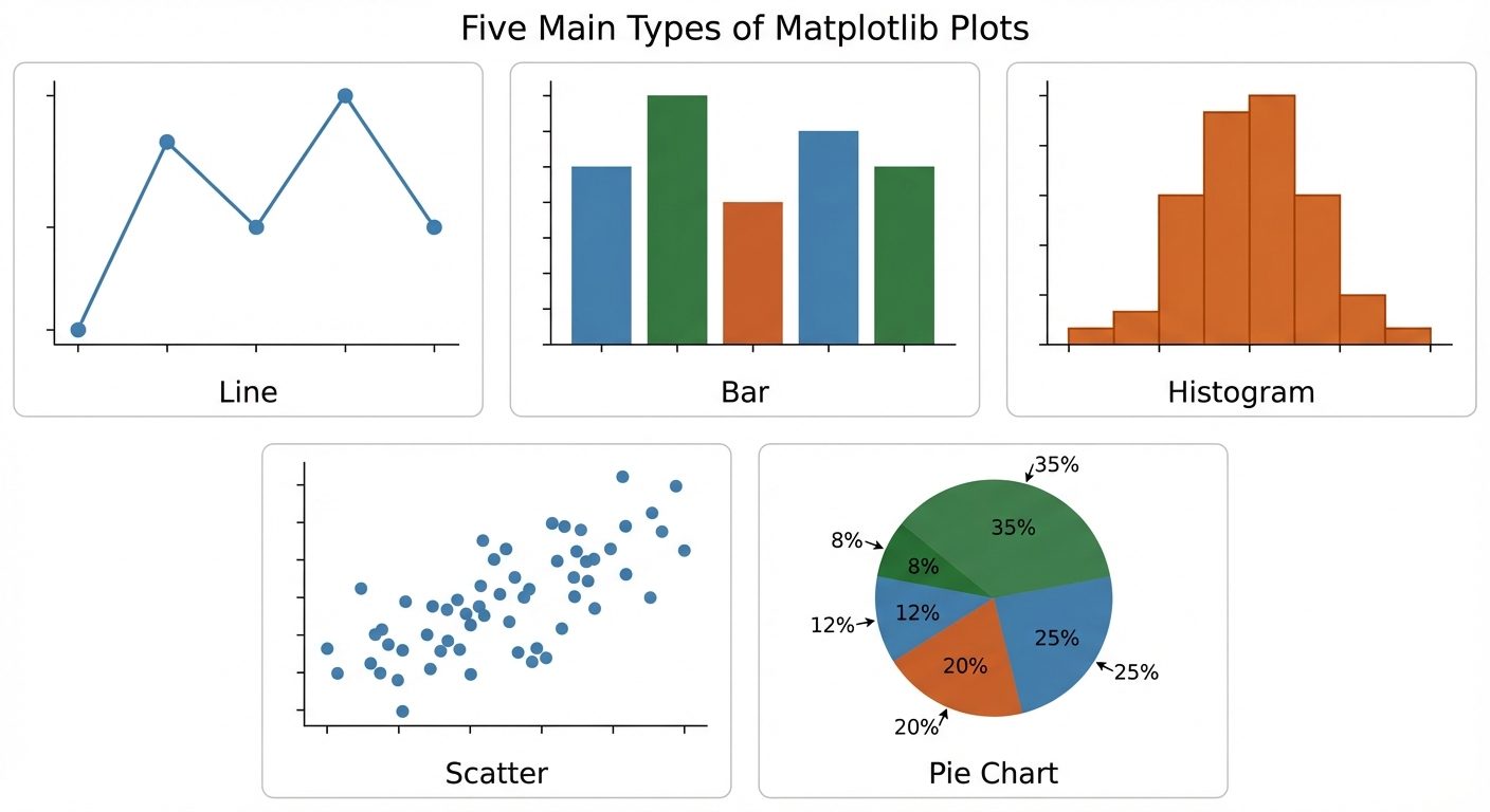
5. Data Visualization using Matplotlib

Matplotlib is a low-level graph plotting library in Python that serves as a visualization utility.

Importing:

import matplotlib.pyplot as plt

5.1 Line Plot

Used to visualize trends over time or sequential data.

x = [1, 2, 3, 4, 5]
y = [2, 4, 6, 8, 10]

plt.plot(x, y, color='green', linestyle='--', marker='o')
plt.title("Line Plot Example")
plt.xlabel("X Axis")
plt.ylabel("Y Axis")
plt.show()

5.2 Bar Plot

Used to compare categorical data.

categories = ['A', 'B', 'C']
values = [10, 20, 15]

plt.bar(categories, values, color='skyblue')
plt.title("Bar Plot Example")
plt.show()

5.3 Histogram

Used to visualize the frequency distribution of a continuous variable.

ages = [22, 55, 62, 45, 21, 22, 34, 42, 42, 4, 99, 102]
bins = [0, 20, 40, 60, 80, 100]

plt.hist(ages, bins, histtype='bar', rwidth=0.8)
plt.title("Age Distribution")
plt.show()

5.4 Scatter Plot

Used to observe relationships/correlations between two numeric variables.

x = [5, 7, 8, 7, 2, 17, 2, 9]
y = [99, 86, 87, 88, 111, 86, 103, 87]

plt.scatter(x, y, c='red')
plt.title("Scatter Plot")
plt.show()

5.5 Pie Chart

Used to display proportions of a whole.

labels = ['Python', 'Java', 'C++']
sizes = [215, 130, 245]

plt.pie(sizes, labels=labels, autopct='%1.1f%%', startangle=140)
plt.axis('equal') # Ensures pie is drawn as a circle
plt.show()

6. Customizing Plots

Customization improves the readability and aesthetics of the plots.

• Titles and Labels:
  
  PYTHON

      plt.title("Global Sales Data")
      plt.xlabel("Year")
      plt.ylabel("Sales ($)")
      

• Legends: Used to identify multiple datasets on the same plot.
  
  PYTHON

      plt.plot(x, y1, label='Company A')
      plt.plot(x, y2, label='Company B')
      plt.legend(loc='upper right')
      

• Grid:
  
  PYTHON

      plt.grid(True, linestyle='--', alpha=0.6)
      

• Colors and Styles:
  • Colors: 'b' (blue), 'g' (green), 'r' (red), 'k' (black).
  • Markers: 'o' (circle), 's' (square), '^' (triangle).
  • Line Styles: '-' (solid), '--' (dashed), ':' (dotted).

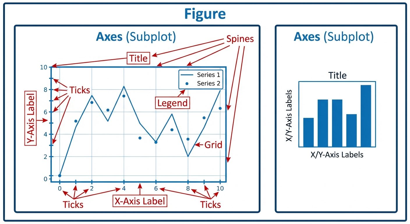
7. Subplots

The subplot() function allows you to draw multiple plots in a single figure (canvas).

Syntax: plt.subplot(nrows, ncols, index)

Example: Creating a 1x2 grid (1 row, 2 columns).

# Plot 1
plt.subplot(1, 2, 1) # (1 row, 2 cols, index 1)
plt.plot(x, y)
plt.title("First Plot")

# Plot 2
plt.subplot(1, 2, 2) # (1 row, 2 cols, index 2)
plt.scatter(x, y)
plt.title("Second Plot")

plt.suptitle("Multiple Plots Example") # Main title for the whole figure
plt.show()

Alternatively, plt.subplots() (plural) creates the figure and axes objects at once:

fig, axes = plt.subplots(nrows=2, ncols=2)
axes[0,0].plot(x, y) # Top left
axes[0,1].bar(x, y)  # Top right
axes[1,0].scatter(x, y) # Bottom left
axes[1,1].hist(y)    # Bottom right
plt.show()