Unit 1: Machine Learning Foundation

1. Introduction to Machine Learning

Machine Learning (ML) is a subfield of artificial intelligence (AI) that focuses on the development of algorithms and statistical models that enable computers to perform tasks without explicit instructions, relying instead on patterns and inference.

• Formal Definition (Tom Mitchell): "A computer program is said to learn from experience E with respect to some class of tasks T and performance measure P, if its performance at tasks in T, as measured by P, improves with experience E."
• Key Concept: Instead of hard-coding rules (if-then-else), the system learns the rules from data.

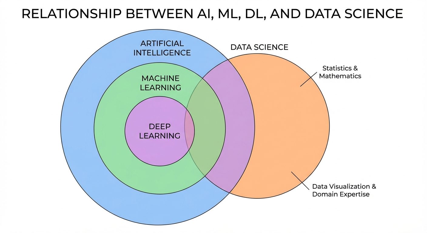
2. AI vs. Machine Learning vs. Data Science

Understanding the boundaries and overlaps between these fields is crucial.

• Artificial Intelligence (AI): The broad concept of creating smart machines capable of performing tasks that typically require human intelligence.
• Machine Learning (ML): A subset of AI. It provides the statistical tools to explore, analyze, and understand data. It is the engine that drives modern AI.
• Data Science (DS): An interdisciplinary field that uses scientific methods, processes, algorithms, and systems to extract knowledge from data. It intersects with AI and ML but also includes data visualization, data engineering, and domain expertise.

3. Types of Machine Learning

Machine learning algorithms are generally categorized based on how they learn (the nature of the "signal" or "feedback" available to the learning system).

A. Supervised Learning

The model is trained on a labeled dataset. The algorithm learns the mapping function from input variables () to output variables ().

• Goal: Predict the output for new, unseen data.
• Sub-categories:
  • Classification: Output is a category (e.g., Spam or Not Spam).
  • Regression: Output is a continuous value (e.g., predicting house prices).

B. Unsupervised Learning

The model is trained on an unlabeled dataset. The system tries to learn the patterns and structure from the data without any teacher.

• Goal: Discover hidden structures in data.
• Sub-categories:
  • Clustering: Grouping similar data points (e.g., Customer Segmentation).
  • Dimensionality Reduction: Reducing the number of variables while keeping the underlying trend (e.g., PCA).

C. Reinforcement Learning (RL)

An agent interacts with an environment and learns to perform actions to maximize cumulative rewards.

• Components: Agent, Environment, Action, State, Reward.
• Mechanism: Trial and error (e.g., AlphaGo, Robot Navigation).

4. Model Categorizations

Parametric vs. Non-parametric Models

• Parametric Models:
  • Definition: Algorithms that simplify the function to a known form with a fixed number of parameters, regardless of the amount of data.
  • Examples: Linear Regression, Logistic Regression.
  • Pros: Fast, require less data.
  • Cons: Limited flexibility, simpler assumptions may not fit complex data.
• Non-parametric Models:
  • Definition: Algorithms that do not make strong assumptions about the form of the mapping function. The number of parameters grows with the amount of data.
  • Examples: K-Nearest Neighbors (KNN), Decision Trees, SVM.
  • Pros: Flexible, can model complex patterns.
  • Cons: Slower, require more data, higher risk of overfitting.

Generative vs. Discriminative Models

• Discriminative Models: Learn the decision boundary between classes. They model the conditional probability .
  • Analogy: Learning the difference between a dog and a cat by looking at their features.
  • Examples: Logistic Regression, SVM.
• Generative Models: Learn the distribution of individual classes. They model the joint probability (and can derive ). They can generate new data instances.
  • Analogy: Learning what a dog looks like and what a cat looks like separately.
  • Examples: Naive Bayes, GANs (Generative Adversarial Networks).

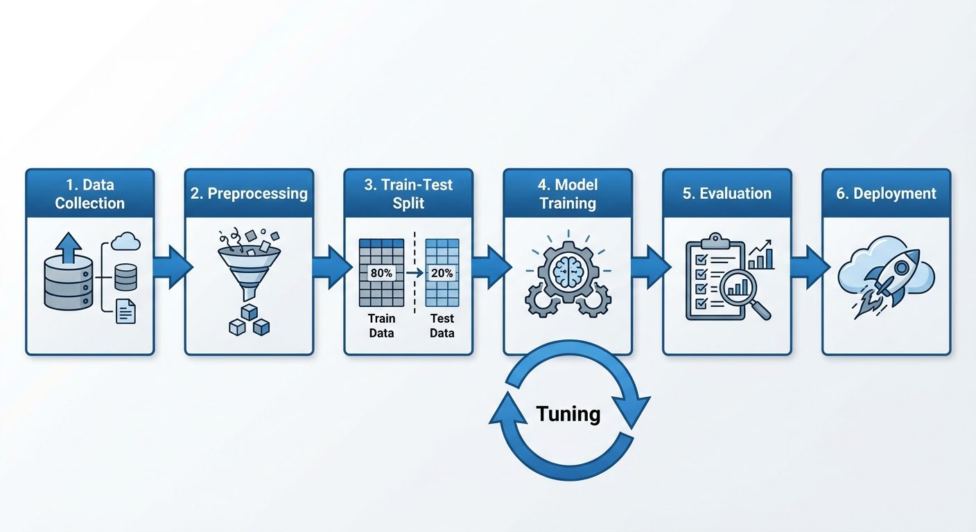
5. Machine Learning Workflow

Building a successful ML model requires a systematic approach.

1. Problem Definition: clearly defining the goal (e.g., "Predict customer churn").
2. Data Collection: Gathering raw data from various sources (DBs, APIs, Sensors).
3. Data Preprocessing: Cleaning data, handling missing values, encoding categorical variables, and scaling features.
4. Data Splitting: separating data into training and testing sets.
5. Model Selection & Training: Choosing an algorithm and fitting it to the training data.
6. Evaluation: Measuring performance using metrics on the test set.
7. Hyperparameter Tuning: Optimizing model settings.
8. Deployment: Integrating the model into a production environment.

6. Evaluation and Performance

Train-Test Split

To verify that a model can generalize to unseen data, the dataset is split:

• Training Set (70-80%): Used to train the model.
• Test Set (20-30%): Used to evaluate performance. Never used during training.

Overview of Evaluation Metrics

• For Classification:
  • Accuracy: Correct Predictions / Total Predictions.
  • Precision: TP / (TP + FP) (How many selected items are relevant?).
  • Recall: TP / (TP + FN) (How many relevant items are selected?).
  • F1-Score: Harmonic mean of Precision and Recall.
• For Regression:
  • MAE (Mean Absolute Error): Average of absolute errors.
  • MSE (Mean Squared Error): Average of squared errors (penalizes large errors).
  • RMSE: Square root of MSE.

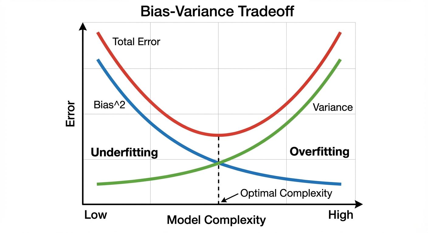
Overfitting and Underfitting

• Underfitting (High Bias): The model is too simple to capture the underlying pattern of the data. It performs poorly on both training and test data.
• Overfitting (High Variance): The model is too complex and learns the noise in the training data rather than the signal. It performs well on training data but poorly on test data.
• Good Fit: The model balances bias and variance, performing well on both datasets.

Bias-Variance Trade-off

• Bias: Error due to overly simplistic assumptions in the learning algorithm.
• Variance: Error due to too much complexity in the learning algorithm (sensitivity to small fluctuations in the training set).
• Trade-off: As you increase model complexity, bias decreases but variance increases. The goal is to find the "sweet spot" where the Total Error is minimized.

7. Applications and Use-cases

• Healthcare: Disease diagnosis, drug discovery, personalized treatment.
• Finance: Fraud detection, credit scoring, algorithmic trading.
• Retail/E-commerce: Recommender systems (Amazon/Netflix), inventory management.
• Transportation: Self-driving cars, route optimization (Google Maps).
• NLP: Chatbots, translation, sentiment analysis.

8. Numpy for Numerical Computing

NumPy (Numerical Python) is the foundational library for scientific computing in Python. It provides support for large, multi-dimensional arrays and matrices, along with a collection of mathematical functions to operate on them.

Why Numpy?

• Speed: Written in C, optimized for vectorization (avoids slow Python loops).
• Memory Efficiency: Uses contiguous blocks of memory.

Creating Arrays

import numpy as np

# From a list
arr = np.array([1, 2, 3])

# 2D Array (Matrix)
matrix = np.array([[1, 2, 3], [4, 5, 6]])

# Built-in functions
zeros = np.zeros((3, 3))       # 3x3 matrix of zeros
ones = np.ones((2, 4))         # 2x4 matrix of ones
arange = np.arange(0, 10, 2)   # [0, 2, 4, 6, 8]
linspace = np.linspace(0, 1, 5) # 5 values equally spaced between 0 and 1

Operations on Arrays

Operations are element-wise by default.

a = np.array([1, 2, 3])
b = np.array([4, 5, 6])

sum_val = a + b      # [5, 7, 9]
prod_val = a * b     # [4, 10, 18]
scalar_op = a * 2    # [2, 4, 6]

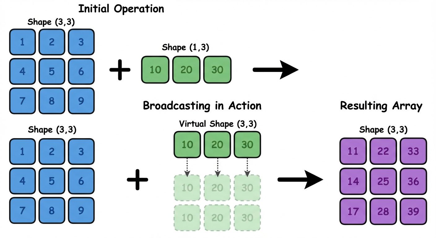
Broadcasting Rule

Broadcasting allows NumPy to perform arithmetic operations on arrays of different shapes.

• Rule: Two dimensions are compatible when:
  1. They are equal, or
  2. One of them is 1.
• If compatible, the smaller array is "stretched" to match the larger array's shape.

Matrix Operations

For linear algebra, we use dot products, not element-wise multiplication.

A = np.array([[1, 2], [3, 4]])
B = np.array([[5, 6], [7, 8]])

# Matrix Multiplication (Dot Product)
result = np.dot(A, B)
# OR using the @ operator
result_2 = A @ B 

# Transpose
A_trans = A.T

Random Module

Used for initializing weights in neural networks or splitting data.

# Random float between 0 and 1
rand_num = np.random.rand()

# Array of random floats
rand_arr = np.random.rand(3, 2)

# Random integers between low and high
rand_int = np.random.randint(0, 10, size=(5,))

# Setting a seed for reproducibility
np.random.seed(42)