Unit 4: Graphs theory I

1. Graph Terminologies

A Graph consists of a set of vertices (nodes) and a set of edges connecting pairs of vertices.

• Directed Graph (Digraph): Edges have direction (ordered pairs).
• Undirected Graph: Edges have no direction (unordered pairs).
• Loop: An edge connecting a vertex to itself.
• Parallel Edges (Multi-graph): Multiple edges connecting the same pair of vertices.
• Simple Graph: A graph with no loops and no parallel edges.
• Degree of a Vertex (): The number of edges incident to a vertex.
  • Isolated Vertex: Degree = 0.
  • Pendant Vertex: Degree = 1.
  • Handshaking Theorem: . (Sum of degrees is twice the number of edges).
• In-Degree / Out-Degree (Digraphs):
  • : Number of edges entering .
  • : Number of edges leaving .
  • .

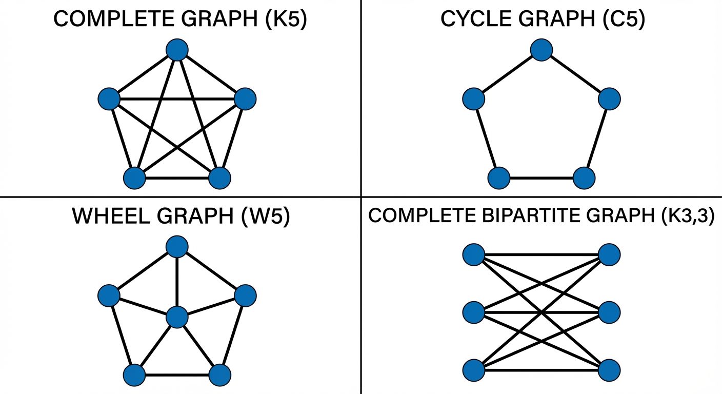
2. Special Types of Graphs

• Complete Graph (): A simple graph where every pair of distinct vertices is connected by a unique edge.
  • Number of edges: .
  • Regularity: -regular.
• Cycle Graph (): A closed loop of vertices () and edges.
• Wheel Graph (): Formed by adding a center vertex to a cycle and connecting it to all vertices in the cycle. Total vertices: .
• Regular Graph: Every vertex has the same degree (-regular).
• Cube (Hypercube ): Vertices represent -bit strings. Two vertices are connected if their strings differ by exactly one bit.
• Bipartite Graph: Vertex set can be partitioned into two disjoint sets and such that every edge connects a vertex in to one in . No edges exist within or within .
• Complete Bipartite Graph (): Every vertex in set (size ) is connected to every vertex in set (size ).

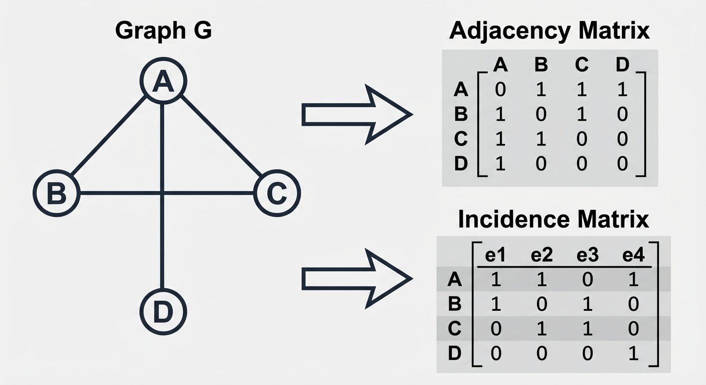
3. Representing Graphs

Adjacency Matrix ()

A square matrix of size (where ).

• if there is an edge from to .
• otherwise.
• For undirected graphs, the matrix is symmetric.

Incidence Matrix ()

A matrix of size (Vertices Edges).

• if edge is incident on vertex .
• otherwise.

Adjacency List

An array of lists where the -th list contains the neighbors of vertex . More space-efficient for sparse graphs.

4. Graph Isomorphism

Two graphs and are isomorphic if there exists a one-to-one and onto function (bijection) that preserves adjacency.

Necessary Conditions (Invariants):
For graphs to be isomorphic, they must have the same:

1. Number of vertices.
2. Number of edges.
3. Degree sequence (list of degrees sorted in non-increasing order).

Note: These conditions are necessary but not sufficient.

5. Path and Connectivity

Definitions

• Walk: Alternating sequence of vertices and edges.
• Trail: A walk with no repeated edges.
• Path: A walk with no repeated vertices.
• Circuit: A closed trail (starts and ends at same vertex).
• Cycle: A closed path (starts and ends at same vertex, no other repeats).

Connectivity in Undirected Graphs

• Connected Graph: There is a path between every pair of distinct vertices.
• Cut Vertex (Articulation Point): A vertex whose removal increases the number of connected components.
• Cut Edge (Bridge): An edge whose removal increases the number of connected components.

Connectivity in Digraphs

• Strongly Connected: For every pair , there is a directed path AND .
• Weakly Connected: The underlying undirected graph (ignoring direction) is connected.

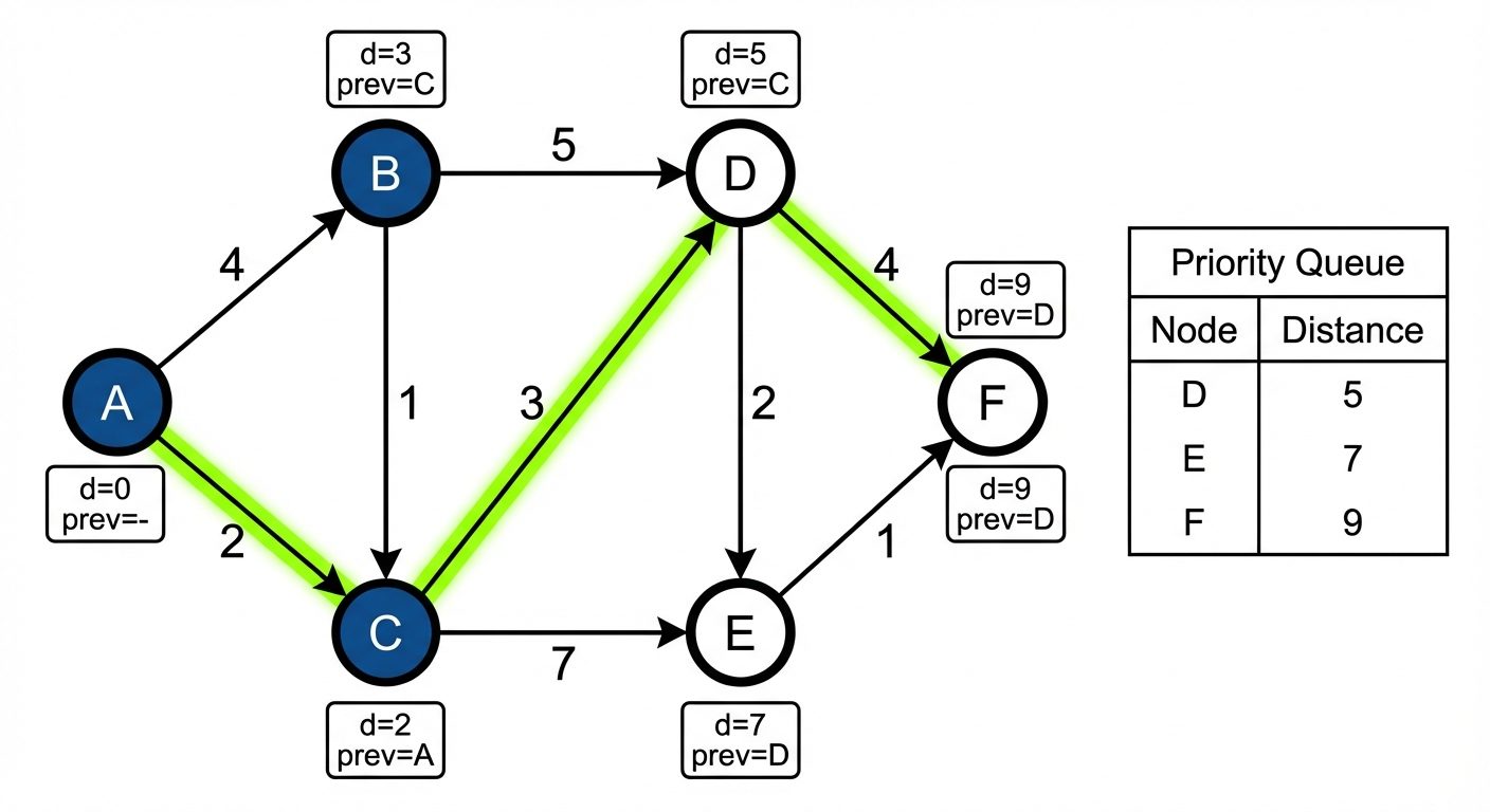
6. Dijkstra’s Algorithm (Shortest Path)

Used to find the shortest path from a source node to all other nodes in a weighted graph (weights must be non-negative).

The Algorithm (Greedy Approach)

1. Initialization:
   • Set distance to source = 0.
   • Set distance to all other nodes = .
   • Mark all nodes as unvisited.
2. Selection: Select the unvisited node with the smallest tentative distance (call it u).
3. Relaxation:
   • For each unvisited neighbor v of u:
     • Calculate new_dist = distance(u) + weight(u, v).
     • If new_dist < distance(v), update distance(v) = new_dist.
4. Termination: Mark u as visited. Repeat steps 2-4 until the destination is visited or all reachable nodes are processed.

Complexity

• with simple array.
• with priority queue.