Practical 4: Application of GIS for Environment Degradation

1. Aim/Objective

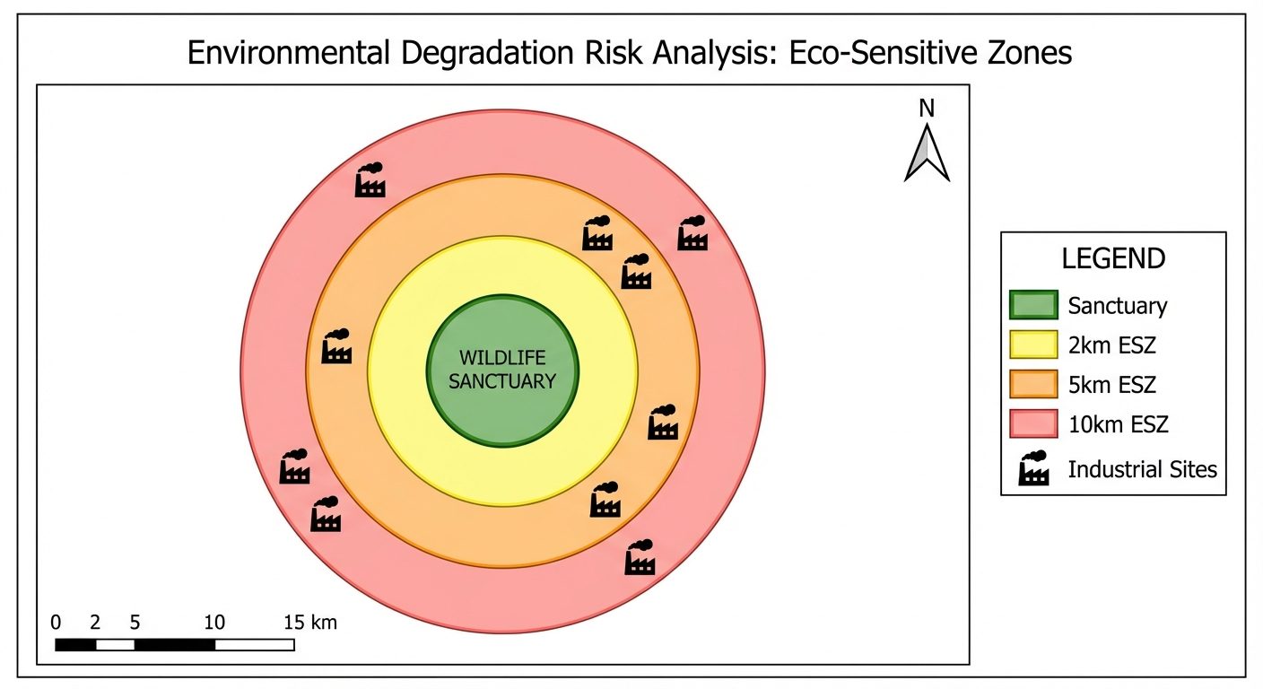
To apply Spatial Analysis techniques in a Geographic Information System (GIS) environment to assess environmental degradation by creating Eco-Sensitive Zones (ESZ) using Multi-Ring Buffers around a Wildlife Sanctuary and identifying overlapping or conflicting Industrial Zones.

2. Apparatus/Components Required

• Hardware: Personal Computer/Laptop with minimum 8GB RAM, multi-core processor, and standard pointing device (mouse).
• Software: QGIS (Quantum GIS) version 3.x OR ESRI ArcGIS Pro / ArcMap 10.x.
• Data Sets (Vector Data):
  • Wildlife_Sanctuary.shp (Polygon shapefile representing the boundary of the protected area)
  • Industrial_Zones.shp (Point/Polygon shapefile representing locations and extents of factories/industries)
  • Admin_Boundary.shp (Polygon shapefile for base map reference)

3. Theory

Environmental Degradation and GIS:
Environmental degradation occurs when the environment is compromised through the depletion of resources such as air, water, and soil, leading to the destruction of ecosystems. GIS serves as a powerful spatial decision-support tool to monitor, map, and analyze these degrading factors.

Eco-Sensitive Zones (ESZ):
ESZs act as "shock absorbers" for protected areas. They are transitional areas around National Parks and Wildlife Sanctuaries where heavily polluting human activities and industries are restricted or highly regulated.

Multi-Ring Buffer Analysis:
Buffering is a geoprocessing tool that creates polygons at a specified distance around an input feature. A Multi-Ring Buffer generates multiple concentric polygons at specific distance intervals (e.g., 2 km, 5 km, 10 km). This is highly useful for categorizing risk zones:

• High Risk / Highly Sensitive: 0 - 2 km from the sanctuary.
• Moderate Risk: 2 - 5 km from the sanctuary.
• Low Risk: 5 - 10 km from the sanctuary.

By overlaying Industrial Zones with these buffers via spatial intersection, we can quantify environmental threats.

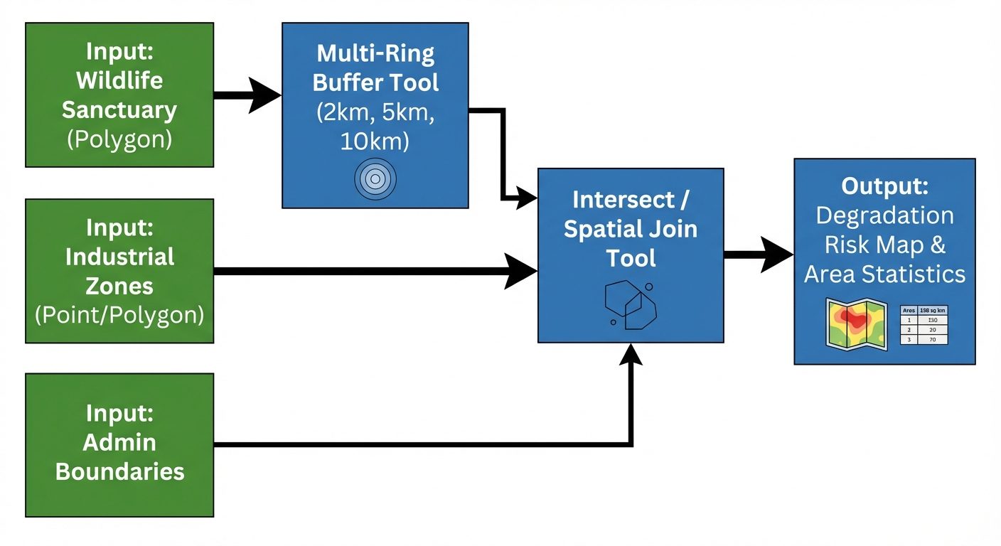
4. Circuit Diagram / Setup (GIS Workflow Architecture)

In a software-based GIS practical, the "Circuit Setup" translates to the Geoprocessing Workflow and Software UI Setup.

5. Procedure

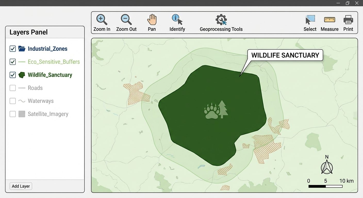
Step 1: Workspace Setup and Data Loading

1. Launch the GIS software (e.g., QGIS).
2. Start a New Project and set the Project Coordinate Reference System (CRS) to a Projected Coordinate System (e.g., WGS 84 / UTM zone relevant to the study area). Note: Projected CRS is mandatory for accurate distance calculations in meters/kilometers.
3. Go to Layer > Add Layer > Add Vector Layer. Browse and add Wildlife_Sanctuary.shp and Industrial_Zones.shp.

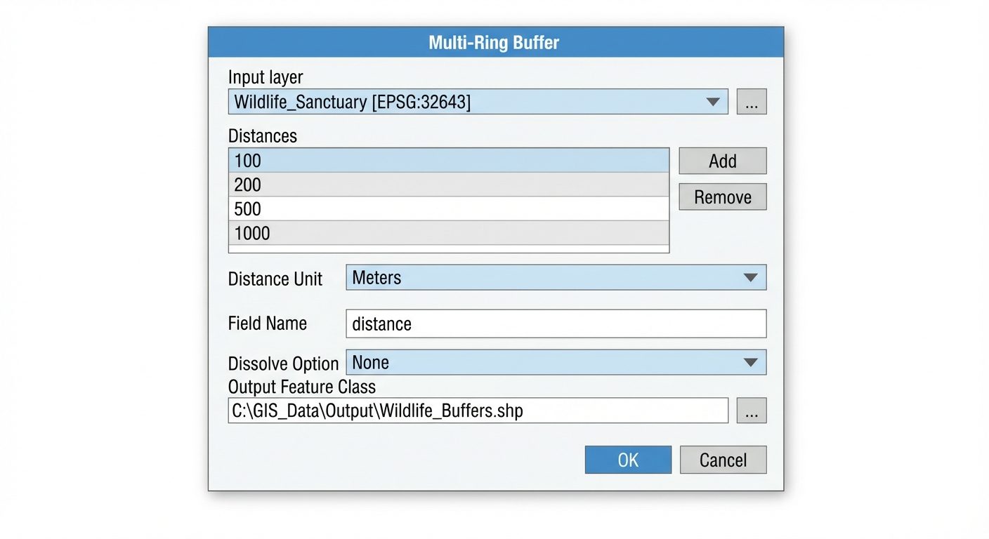
Step 2: Creation of Multi-Ring Buffers (Eco-Sensitive Zones)

1. Open the Processing Toolbox (Ctrl+Alt+T in QGIS).
2. Search for and open the Multi-ring buffer (constant distance) tool.
3. Set the parameters:
   • Input Layer: Wildlife_Sanctuary.shp
   • Number of rings: 3
   • Distance between rings: 2000, 3000, 5000 (to create 2km, 5km, and 10km cumulative rings assuming CRS is in meters).
   • Check the option to Dissolve results so overlapping boundaries merge into continuous rings.
4. Click Run. A new temporary layer named Multi-ring buffer will be generated.

" selected. Below it, a "Distances" text field containing "2000, 5000, 10000". A checkbox labeled "Dissolve result" which is checked. A "Run" button at the bottom right. The layout should mimic standard GIS geoprocessing parameter windows with a grey background and clean black text.]

Step 3: Symbology and Visualization

1. Right-click the newly created buffer layer and select Properties > Symbology.
2. Change the styling to Categorized, select the buffer distance field, and apply a color ramp (e.g., Red for 2km, Orange for 5km, Yellow for 10km).
3. Ensure the Wildlife_Sanctuary.shp layer is placed on top of the buffer layer in the Layers Panel.

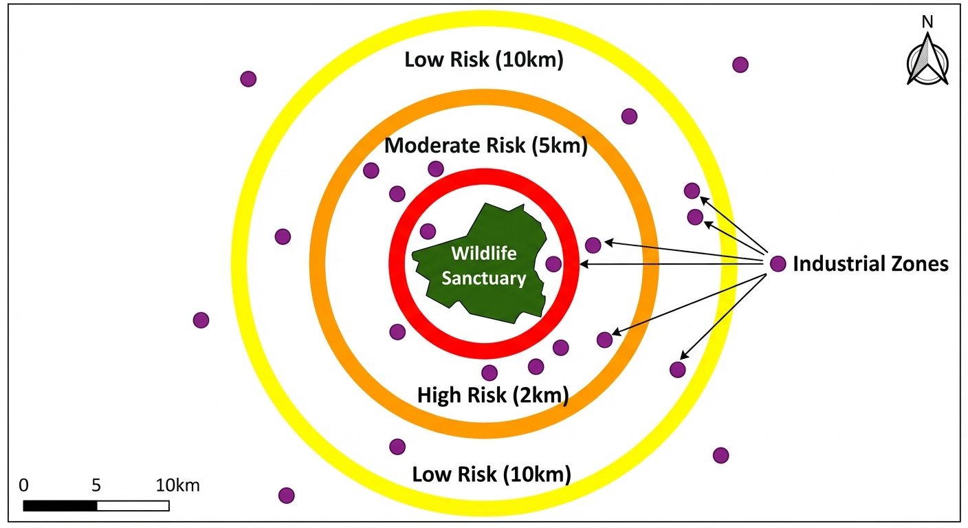
Step 4: Overlay Analysis (Identifying Environment Degradation Threats)

1. To find out which industries are violating the Eco-Sensitive Zones, open the Intersection tool (Vector > Geoprocessing Tools > Intersection).
2. Set Input Layer as Industrial_Zones.shp.
3. Set Overlay Layer as the newly created Multi-ring buffer layer.
4. Click Run. A new layer (Intersected_Industries) is created, containing only the industries situated within the buffer zones, appending the buffer distance data to each industry's attribute.

Step 5: Attribute Analysis and Area Calculation

1. Open the Attribute Table of the Intersected_Industries layer to count the number of degraded zones.
2. Open the Attribute Table of the Multi-ring buffer layer to calculate the total area of the ESZ.

6. Observations / Truth Tables / Readings

Table 1: Eco-Sensitive Zone (Buffer) Area Matrix
This "truth table" equivalent shows the calculated areas for each risk zone generated by the Multi-Ring Buffer.

Zone Category	Buffer Distance (km)	Area (Sq. km)	Sensitivity Level
Core	0 (Inside Sanctuary)	124.50	Protected
Tier 1	0 - 2	45.20	Extremely High Risk
Tier 2	2 - 5	88.60	High Risk
Tier 3	5 - 10	165.30	Moderate Risk

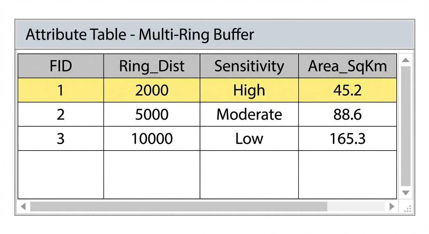
Table 2: Industrial Encroachment Intersect Observations
Analysis of industries falling within the restricted zones.

Industrial Zone ID	Industry Type	Distance to Sanctuary boundary	Zone Violation	Status
IND-042	Chemical	1.2 km	Tier 1 (0-2 km)	High Threat / Legal Violation
IND-088	Textile	3.5 km	Tier 2 (2-5 km)	Monitored
IND-105	Cement	1.8 km	Tier 1 (0-2 km)	High Threat / Legal Violation
IND-201	Manufacturing	8.2 km	Tier 3 (5-10 km)	Safe/Permitted

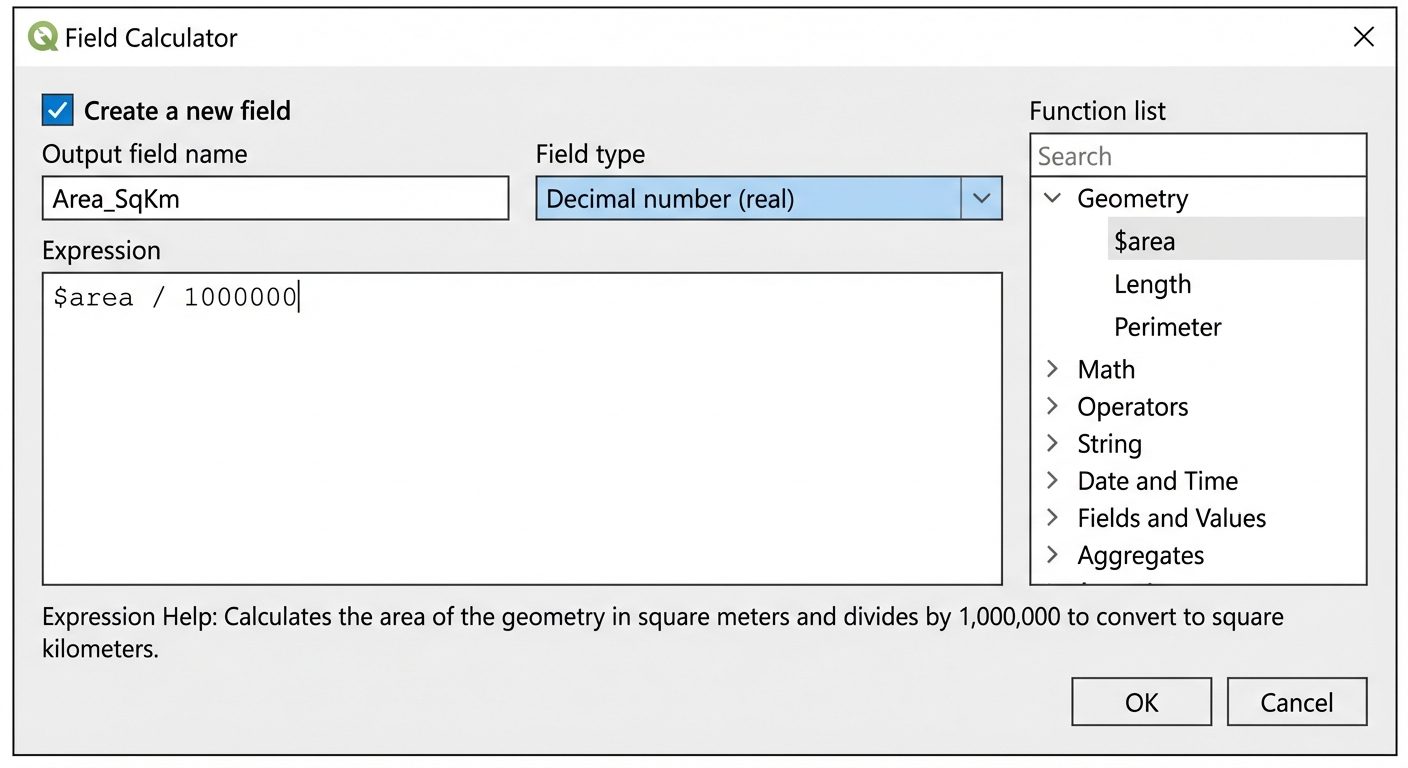
7. Calculations

To calculate the spatial extent of the degraded zones (ESZ area):

1. In the buffer layer's Attribute Table, click Open Field Calculator (Ctrl+I).
2. Create a new field:
   • Output field name: Area_SqKm
   • Output field type: Decimal number (real)
3. Enter the geometry expression for calculating area in Square Kilometers (assuming map units are meters):
   
   TEXT

      $area / 1000000
      

4. Click OK. The new column will populate with the area of each buffer ring.

8. Result

The Multi-Ring Buffer spatial analysis was successfully performed. Three tiers of Eco-Sensitive Zones (2km, 5km, and 10km) were delineated around the Wildlife Sanctuary. Overlay analysis with the Industrial Zones identified 2 industries operating within the high-threat 2km zone, indicating severe environmental degradation risk and potential violation of environmental protection laws. The final thematic map layout containing legends, scale, and north arrow was successfully exported.

9. Viva Questions

1. What is a Buffer in GIS?
   Answer: A buffer is a proximity analysis tool that creates a zone (polygon) of a specified distance around a point, line, or polygon feature to identify areas of influence or restriction.
2. What is the difference between a standard Buffer and a Multi-Ring Buffer?
   Answer: A standard buffer creates a single boundary at one fixed distance. A Multi-Ring Buffer creates multiple, concentric polygons at varying specified intervals (e.g., 1km, 2km, 3km) simultaneously.
3. Why must we use a Projected Coordinate System (like UTM) instead of a Geographic Coordinate System (like WGS 84) when generating buffers?
   Answer: Geographic Coordinate Systems measure in degrees, which do not translate to uniform distances across the globe. Projected systems measure in linear units (meters/feet), allowing accurate buffering in kilometers.
4. What does the 'Dissolve' function do during buffer generation?
   Answer: The dissolve function merges overlapping boundaries of overlapping buffer zones into a single continuous polygon, preventing duplicated overlapping areas in calculations.
5. Which Geoprocessing tool is best for finding out which specific industries fall inside the newly created 2km buffer zone?
   Answer: The 'Intersect' tool or 'Spatial Join' tool. Intersect will output only the industrial zones that fall within the buffer, combining attributes of both layers.
6. In the Field Calculator, what does the expression $area compute?
   Answer: $area computes the geometric area of the polygon feature in the native units of the layer's coordinate reference system (usually square meters).
7. How does GIS aid in assessing Environmental Degradation?
   Answer: GIS allows for the spatial mapping of sensitive areas (forests, water bodies) and degrading factors (industries, deforestation). Overlay analysis helps quantify the extent of damage and identifies zones requiring immediate policy intervention.