Practical 3
Practical 3: Land use /land Cover Change Detection
1. Aim/Objective
To perform spatial and temporal analysis on multi-spectral satellite imagery to detect, quantify, and map the Land Use / Land Cover (LULC) changes over a specific time period using Geographical Information System (GIS) techniques.
2. Apparatus/Components Required
- Hardware: A high-performance computer/workstation with sufficient RAM (minimum 8GB, 16GB recommended) and a multi-core processor.
- Software: QGIS (Quantum GIS) v3.x or ESRI ArcGIS Pro / ArcMap 10.x.
- Plugins/Extensions: Semi-Automatic Classification Plugin (SCP) for QGIS or Spatial Analyst Extension for ArcGIS.
- Data/Inputs: Multi-temporal satellite imagery of the same geographical extent from two different time periods (e.g., Landsat 8/9 OLI, Sentinel-2). Cloud cover should be less than 10%.
- Ancillary Data: High-resolution Google Earth imagery (for accuracy assessment / ground truthing), shapefile of the Study Area (Area of Interest - AOI).
3. Theory
Land Use/Land Cover (LULC):
- Land Cover refers to the physical material at the surface of the earth (e.g., grass, asphalt, trees, bare ground, water).
- Land Use refers to how humans utilize the land (e.g., urban, agricultural, recreational).
Change Detection:
Change detection is the process of identifying differences in the state of an object or phenomenon by observing it at different times. In GIS and remote sensing, it involves analyzing spatial and temporal changes in LULC.
Spatial and Temporal Analysis:
- Spatial Analysis: Examining the geographic distribution and spatial relationships of LULC classes.
- Temporal Analysis: Comparing data across a timeline to observe trends (e.g., urbanization, deforestation) over and .
Post-Classification Comparison:
The most common method for LULC change detection. It involves classifying the multi-temporal images independently and then comparing the classified maps pixel-by-pixel to create a transition matrix and a change map.
4. Setup / Workflow Diagram
To properly execute this practical, the spatial analysis workflow must be structured correctly within the GIS environment.
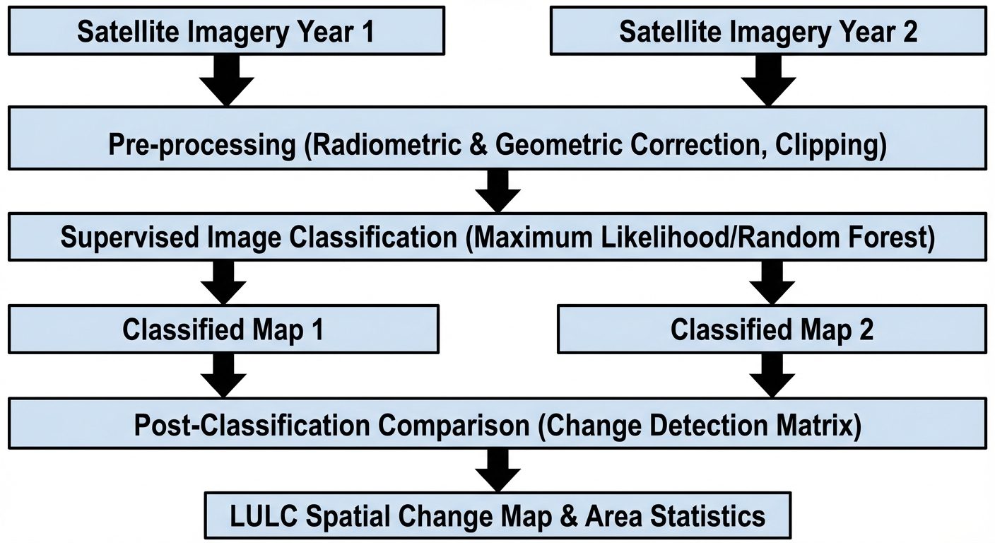
5. Procedure
Step 1: Data Acquisition and Pre-processing
- Download multi-spectral satellite imagery for Time 1 () and Time 2 () from sources like USGS EarthExplorer.
- Load the imagery bands into the GIS software.
- Perform layer stacking to create composite multi-spectral images for both and .
- Clip/Mask the stacked rasters using the Area of Interest (AOI) shapefile to limit the processing area.
Step 2: Creation of Training Samples (Signatures)
- Open the Image Classification toolbar (or SCP plugin).
- Create training polygons (Regions of Interest - ROIs) for at least 4-5 classes (e.g., Water Bodies, Vegetation, Built-up/Urban, Agriculture, Bare Land).
- Ensure training samples are evenly distributed across the study area for both images.
- Merge the ROIs to create a signature file for and .
Step 3: Supervised Classification
- Run a Supervised Classification algorithm (e.g., Maximum Likelihood, Random Forest, or Support Vector Machine) using the respective signature files.
- Apply the classification to both and images to generate two independent LULC maps.
- Assign standard color codes to the classes (e.g., Blue for Water, Red for Built-up).
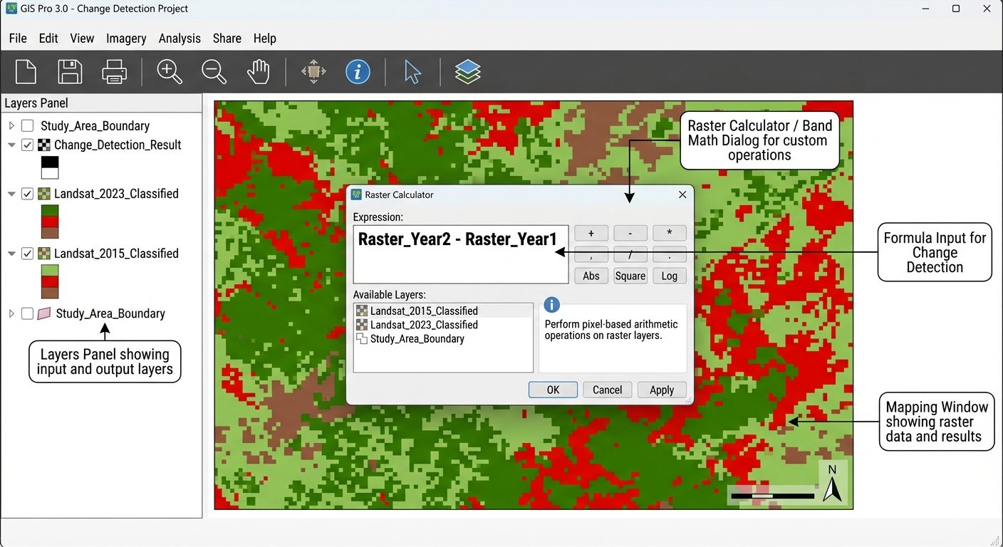
Step 4: Post-Classification Change Detection
- Open the raster cross-tabulation tool (e.g., Combine tool, Tabulate Area tool, or SCP Change Detection tab).
- Input the classified map as the "Reference" or "Initial state" raster.
- Input the classified map as the "New state" raster.
- Execute the tool to generate a Change/Transition Matrix and a Spatial Change Detection Map.
Step 5: Map Composition and Export
- Go to the Print Layout / Layout View.
- Add necessary map elements: Title, North Arrow, Scale Bar, Legend, and Grid.
- Export the final LULC maps and the Change Detection Map as high-resolution images (JPEG/PNG) or PDFs.
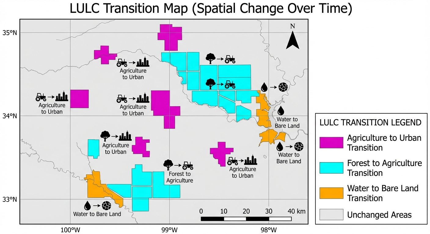
6. Observations / Tables (Transition Matrix)
Instead of a digital truth table, spatial analysis relies on a Transition/Confusion Matrix to observe temporal changes.
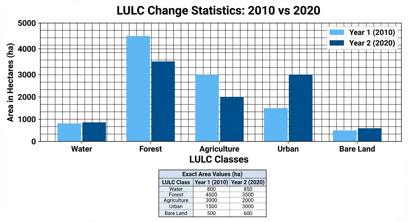
| Table 1: Area Statistics (Hectares) | Class Value | LULC Class | Area Year 1 () | Area Year 2 () | Absolute Change (ha) |
|---|---|---|---|---|---|
| 1 | Water Bodies | 1200.5 | 1150.0 | -50.5 | |
| 2 | Forest | 4500.0 | 3800.2 | -699.8 | |
| 3 | Agriculture | 3100.0 | 2500.8 | -599.2 | |
| 4 | Built-up (Urban) | 850.5 | 2200.0 | +1349.5 | |
| 5 | Bare Land | 349.0 | 349.0 | 0.0 |
Table 2: LULC Transition Matrix ( to ) in Hectares
(Rows = Initial State , Columns = Final State . The diagonal represents unchanged areas).
| \ | Water | Forest | Agriculture | Built-up | Bare Land | Total |
|---|---|---|---|---|---|---|
| Water | 1100.0 | 0.0 | 0.0 | 50.0 | 50.5 | 1200.5 |
| Forest | 0.0 | 3500.0 | 800.0 | 200.0 | 0.0 | 4500.0 |
| Agriculture | 50.0 | 300.2 | 1700.0 | 1049.8 | 0.0 | 3100.0 |
| Built-up | 0.0 | 0.0 | 0.0 | 850.5 | 0.0 | 850.5 |
| Bare Land | 0.0 | 0.0 | 0.8 | 49.7 | 298.5 | 349.0 |
| Total | 1150.0 | 3800.2 | 2500.8 | 2200.0 | 349.0 | 10000.0 |
7. Calculations
1. Area Calculation (if using pixel count):
Example for Landsat (30m resolution):
2. Percentage Change Calculation:
Example for Built-up Area (from Table 1):
8. Result
The spatial and temporal analysis of the multi-spectral satellite imagery was successfully performed.
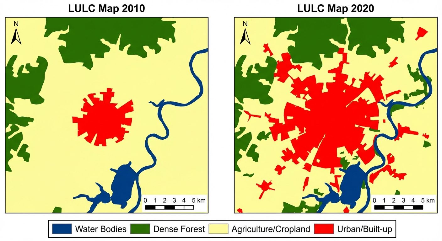
- The LULC Maps for years and were successfully generated using supervised classification.
- The Temporal Analysis reveals significant urbanization. The Built-up area increased by 158.67% (from 850.5 ha to 2200.0 ha).
- The Transition Matrix demonstrates that the majority of this new urban expansion encroached upon agricultural land (1049.8 ha converted from Agriculture to Built-up).
- Forest cover experienced a degradation of approximately 15.5% over the observation period.
9. Viva Questions
Q1. What is the difference between Land Use and Land Cover?
Answer: Land cover refers to the physical or biological cover present on the Earth's surface (e.g., water, vegetation). Land use refers to the human purpose or management applied to that land (e.g., agriculture, residential, commercial).
Q2. What is Post-Classification Comparison in change detection?
Answer: It is a method where two images from different dates are independently classified into LULC categories, and then the resulting maps are overlaid and compared pixel-by-pixel to identify areas of change.
Q3. Why is image pre-processing (radiometric/atmospheric correction) important before LULC classification?
Answer: Pre-processing removes sensor errors, atmospheric scattering, and illumination differences, ensuring that variations in pixel values are due to actual ground changes rather than atmospheric anomalies.
Q4. What is a Transition Matrix (or Cross-tabulation matrix)?
Answer: It is a table showing the relationship between two thematic maps of the same area but from different times. It shows how much area of a specific class in Time 1 remained the same or transitioned into different classes in Time 2.
Q5. How does the spatial resolution of satellite imagery affect LULC mapping?
Answer: Spatial resolution dictates the smallest feature that can be identified. High resolution (e.g., Sentinel 10m) allows for finer LULC classification (individual buildings/roads), while moderate resolution (Landsat 30m) is better for broader regional classification (forest tracts, large agricultural fields).
Q6. What does the Kappa Coefficient signify in image classification?
Answer: The Kappa coefficient is a statistical measure used to assess the accuracy of the image classification. It evaluates how much better the classification performed compared to randomly assigning pixels to classes. A value closer to 1 indicates high accuracy.