Unit 3: Machine Learning

1. Mathematical Foundations for Machine Learning

Machine learning (ML) relies heavily on mathematical concepts to optimize algorithms and process data. An applied understanding of these fields is crucial for implementing ML solutions.

1.1 Applied Linear Algebra

Linear algebra provides the language for manipulating data in high dimensions. In ML, data is rarely processed as single numbers (scalars) but rather as structures.

• Scalars: Single numerical values (0-dimensional tensor).
• Vectors: Ordered arrays of numbers (1-dimensional tensor). A row of data in a dataset (e.g., a specific customer's age, income, and debt) is a vector.
• Matrices: 2-dimensional arrays of numbers. An entire spreadsheet or dataset is a matrix, where rows are samples and columns are features.
• Tensors: N-dimensional arrays (generalization of matrices). Used heavily in Deep Learning (e.g., an RGB image is a rank-3 tensor: Height x Width x Color Channels).

Key Operations:

• Dot Product: A measure of geometric similarity between two vectors. If the dot product is high, the vectors point in a similar direction (are similar).
• Matrix Multiplication: Used to transform data (scaling, rotating) and maps inputs to outputs in Neural Networks.
• Eigenvalues and Eigenvectors: Fundamental in dimensionality reduction techniques like Principal Component Analysis (PCA) to find the "principal directions" of data variance.

1.2 Probability and Statistics

ML deals with uncertainty and stochastic processes. Probability theory quantifies this uncertainty.

• Probability Distribution: Describes how likely different outcomes are.
  • Normal Distribution (Gaussian): The "Bell Curve." Most ML models assume data is normally distributed. Defined by Mean () and Standard Deviation ().
• Mean, Median, Mode: Measures of central tendency.
• Variance and Standard Deviation: Measures of data spread. High variance implies data is scattered widely; low variance implies data is clustered around the mean.
• Correlation vs. Causation: Correlation measures the linear relationship between two variables. ML models exploit correlation to predict outcomes, but this does not imply causation.

2. Types of Machine Learning

Machine Learning is categorized by how the algorithm learns from data.

2.1 Supervised Learning

The algorithm is trained on labeled data. The model learns a mapping function from input variables () to output variables ().

• Goal: Approximation. Find a function such that .
• Sub-categories:
  • Regression: The output variable is continuous/numerical (e.g., predicting house prices, stock values, temperature).
  • Classification: The output variable is categorical (e.g., predicting Spam/Not Spam, Benign/Malignant tumor).
• Real-World Use: Email filtering, credit scoring, voice recognition, medical diagnosis.

2.2 Unsupervised Learning

The algorithm is trained on unlabeled data. The system tries to learn the patterns and structure from the data without an explicit teacher or answer key.

• Goal: Structure discovery.
• Sub-categories:
  • Clustering: Grouping inherent patterns (e.g., K-Means clustering).
  • Dimensionality Reduction: Reducing the number of variables while keeping the principal information (e.g., PCA). Used for visualization and compression.
  • Association: Discovering rules that describe large portions of data (e.g., Market Basket Analysis: "People who buy beer also buy diapers").
• Real-World Use: Customer segmentation, anomaly detection (fraud), recommendation systems (collaborative filtering).

2.3 Reinforcement Learning (RL)

An agent learns to make decisions by performing actions in an environment and receiving feedback in the form of rewards or penalties.

• Key Components:
  • Agent: The learner/decision maker.
  • Environment: The world the agent interacts with.
  • Action: What the agent does.
  • Reward: The feedback signal (positive or negative).
• Concept: The agent aims to maximize the cumulative reward over time (Exploration vs. Exploitation).
• Real-World Use: Robotics (walking, grasping), Game playing (AlphaGo, Chess engines), Self-driving car navigation.

3. Feature Engineering

Feature engineering is the process of using domain knowledge to extract features (characteristics, properties, attributes) from raw data. It is often considered the most critical step in applying ML.

3.1 Feature Selection vs. Extraction

• Feature Selection: Choosing the most relevant subset of existing features. Removing irrelevant features reduces overfitting and improves training speed.
• Feature Extraction: Creating new features from existing ones (e.g., extracting "Day of Week" from a "Timestamp" column, or creating a "Body Mass Index" from "Height" and "Weight").

3.2 Data Preprocessing Techniques

• Handling Missing Data: Strategies include dropping rows (if data is plentiful) or Imputation (filling missing values with the mean, median, or a predicted value).
• Encoding Categorical Data: Machines require numbers, not text.
  • Label Encoding: Assigning a number to each category (Low=0, Mid=1, High=2).
  • One-Hot Encoding: Creating binary columns for each category (Red, Green, Blue become three columns: Is_Red, Is_Green, Is_Blue).
• Feature Scaling: Normalizing the range of independent variables so that one feature (e.g., Salary: 50,000-100,000) doesn't dominate another (e.g., Age: 20-60).
  • Normalization (Min-Max): Scales values between 0 and 1.
  • Standardization (Z-score): Scales data to have a mean of 0 and standard deviation of 1.

4. Model Evaluation

How do we know if a model is "good"? We cannot rely solely on training accuracy, as the model may memorize the data (overfitting).

4.1 Cross-Validation

A technique to assess how the results of a statistical analysis will generalize to an independent dataset.

• K-Fold Cross-Validation:
  1. Split the dataset into equal groups (folds).
  2. For each unique group:
     • Take the group as a hold out or test data set.
     • Take the remaining groups as a training data set.
     • Fit a model on the training set and evaluate it on the test set.
  3. Average the evaluation scores to get the final metric.

4.2 Evaluation Metrics

Accuracy (Correct Predictions / Total Predictions) is often misleading, especially with imbalanced datasets (e.g., fraud detection where 99% of transactions are legitimate).

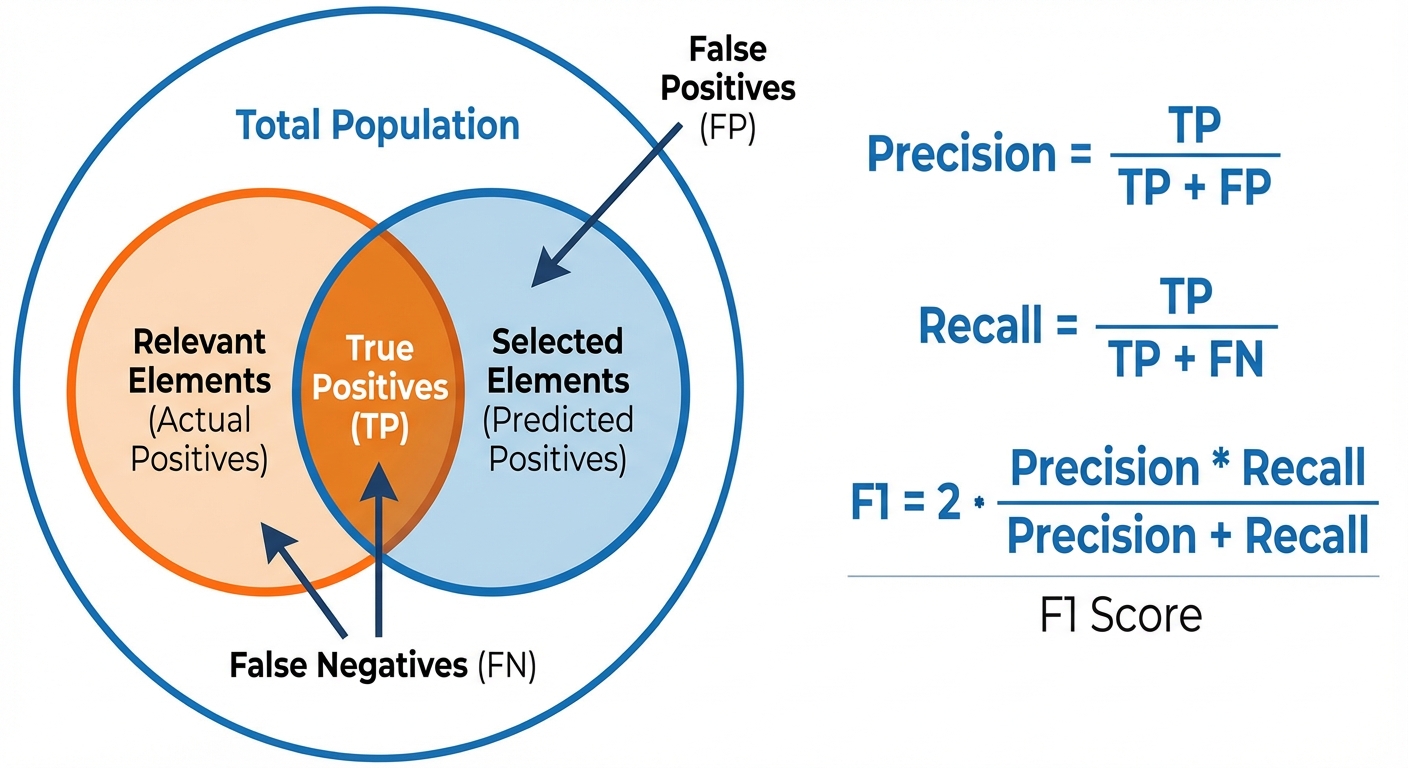
• Confusion Matrix: A table describing the performance of a classification model.
  • True Positive (TP): Correctly predicted positive.
  • True Negative (TN): Correctly predicted negative.
  • False Positive (FP): Incorrectly predicted positive (Type I Error).
  • False Negative (FN): Incorrectly predicted negative (Type II Error).

• Precision: Out of all the instances predicted as positive, how many are actually positive? Useful when the cost of False Positives is high (e.g., email spam detection).
  

• Recall (Sensitivity): Out of all the actual positive instances, how many did the model predict correctly? Useful when the cost of False Negatives is high (e.g., cancer diagnosis).
  

• F1-Score: The harmonic mean of Precision and Recall. Provides a balance between the two.

5. Probabilistic Reasoning

Probabilistic reasoning allows AI systems to make decisions in the presence of uncertainty.

5.1 Bayes' Theorem

Bayes' Theorem describes the probability of an event, based on prior knowledge of conditions that might be related to the event. It is the mathematical formula for updating beliefs based on new evidence.

The Formula:

• (Posterior): The probability of hypothesis A being true given that evidence B has occurred.
• (Likelihood): The probability of evidence B occurring if hypothesis A is true.
• (Prior): The initial probability of hypothesis A being true (before seeing evidence).
• (Evidence): The total probability of the evidence occurring.

Example: Calculating the probability a patient has a disease () given a positive test result (), taking into account the rarity of the disease () and the reliability of the test ().

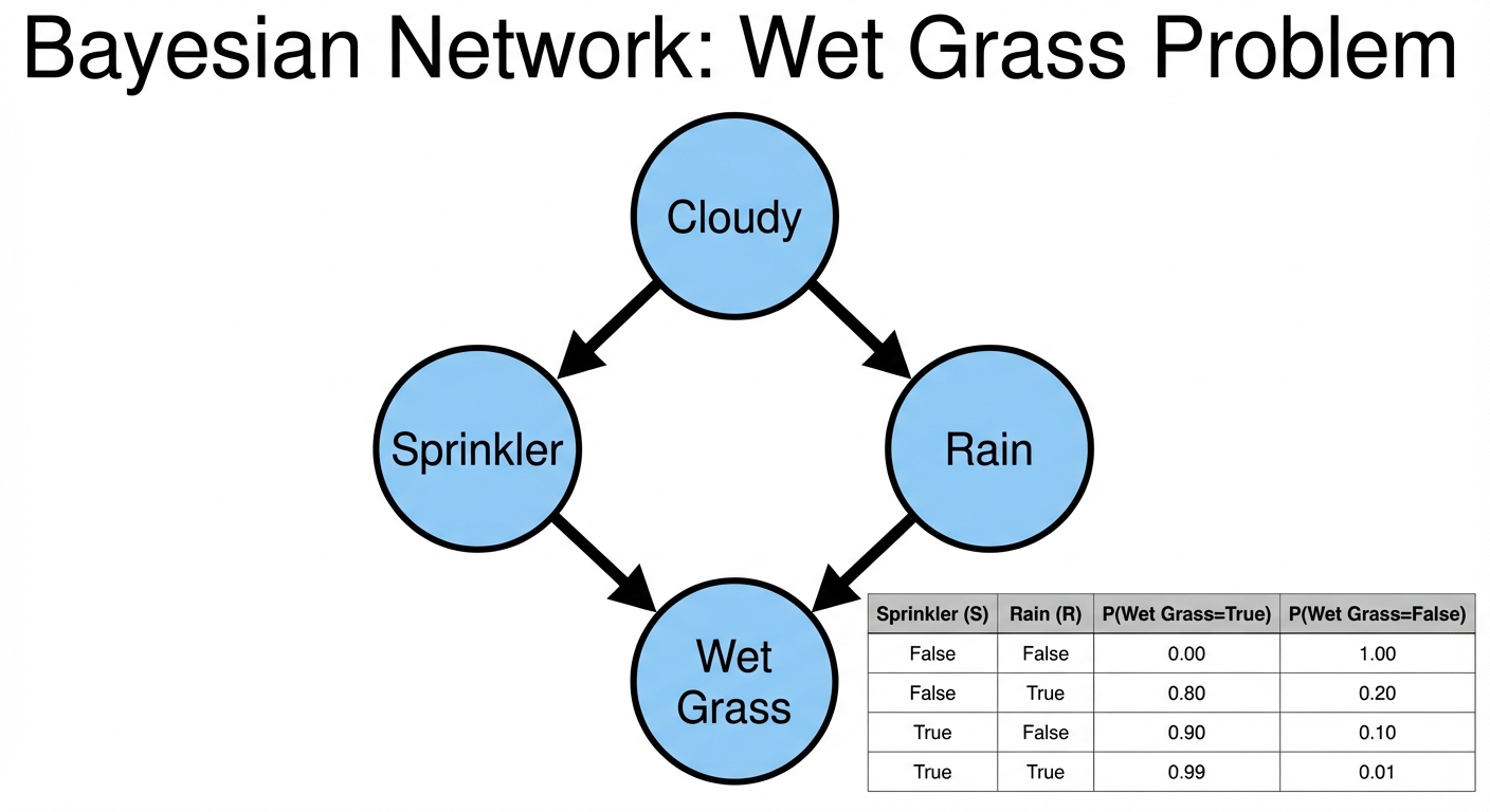
5.2 Bayesian Networks (Belief Networks)

A Bayesian Network is a probabilistic graphical model that represents a set of variables and their conditional dependencies via a Directed Acyclic Graph (DAG).

• Nodes: Represent random variables (e.g., "Rain", "Sprinkler", "Grass Wet").
• Edges: Directed arrows represent causal dependencies. If there is an arrow from Node X to Node Y, X is a "parent" of Y.
• Conditional Probability Table (CPT): Each node has a table quantifying the effect of the parents on the node.

Key Concepts in Bayesian Networks:

• Conditional Independence: A node is independent of its non-descendants given its parents. This property significantly reduces the computational complexity of calculating probabilities.
• Inference: The process of calculating the probability distribution of unobserved variables given observed variables (e.g., Given the grass is wet, what is the probability it rained?).

5.3 Naive Bayes Classifier

A simple but powerful supervised learning algorithm based on Bayes' Theorem.

• "Naive" Assumption: It assumes that all features are mutually independent given the class label. (e.g., In spam detection, the presence of the word "Buy" is independent of the word "Viagra", though both contribute to the probability of "Spam").
• Despite this strong assumption, it performs exceptionally well for text classification and spam filtering.