Unit 2: Problem Solving & Search in AI / AI problem design

1. Problem Formulation and State Space Search

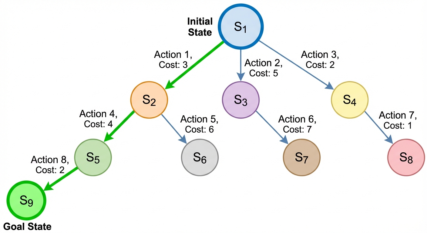
Problem solving in AI is the process of generating a sequence of actions that reaches a goal. Before an agent can start searching for a solution, the problem must be well-defined.

Components of Problem Formulation

To solve a problem computationally, it is modeled using five key components:

1. Initial State: The state in which the agent starts (e.g., the starting city in a route-finding problem).
2. Actions (Description of Operations): The set of possible actions available to the agent. Given a state , returns the set of actions executable in .
3. Transition Model: A description of what each action does. Result() returns the state resulting from doing action in state .
4. Goal Test: Determines whether a given state is a goal state.
5. Path Cost: A numeric cost assigned to each path. The problem-solving agent usually attempts to minimize this cost.

State Space

The State Space is the set of all states reachable from the initial state by any sequence of actions. It forms a directed graph where nodes are states and links are actions.

2. Introduction to Uninformed Search (Blind Search)

Uninformed search algorithms have no additional information about states beyond the problem definition. They do not know if one non-goal state is "better" than another.

Breadth-First Search (BFS)

• Strategy: Expands the shallowest node in the search tree first.
• Data Structure: Uses a First-In-First-Out (FIFO) queue.
• Properties:
  • Complete: Yes (if branching factor is finite).
  • Optimal: Yes (if all step costs are equal).
  • Complexity: Time and Space are (where is branching factor, is depth). High memory consumption is the main drawback.

Depth-First Search (DFS)

• Strategy: Expands the deepest node in the current frontier of the search tree.
• Data Structure: Uses a Last-In-First-Out (LIFO) stack (or recursion).
• Properties:
  • Complete: No (fails in infinite spaces or loops).
  • Optimal: No.
  • Complexity: Time is (where is max depth), but Space is linear . Efficient in memory but dangerous in deep trees.

Uniform Cost Search (UCS)

• Strategy: Expands the node with the lowest path cost .
• Optimal: Yes, for general step costs.
• Mechanism: Equivalent to BFS if all step costs are equal.

3. Core Search Algorithms: Heuristic Search

Informed (Heuristic) search uses domain-specific knowledge to find solutions more efficiently than uninformed search. This knowledge is encoded in a Heuristic Function .

• : Estimated cost of the cheapest path from the state at node to a goal state.
• if is a goal.

Greedy Best-First Search

• Strategy: Expands the node that appears to be closest to the goal.
• Evaluation Function: .
• Pros/Cons: Can be very fast but is not optimal and not complete (can get stuck in loops).

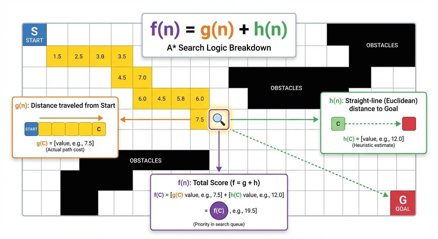
A* Search (A-Star)

The most widely used algorithm in pathfinding. It combines the cost so far with the estimated cost to the goal.

• Evaluation Function:
  • : Actual cost to reach node from the start.
  • : Estimated cost from node to the goal.
• Optimality Conditions:
  1. Admissibility: The heuristic never overestimates the cost to reach the goal ( true cost).
  2. Consistency (Monotonicity): For every node and successor generated by action , .

4. Constraint Satisfaction Problems (CSPs)

CSPs differ from standard search problems by using a factored representation of states.

CSP Components

• Variables (): A set of variables .
• Domains (): A set of domains , where each variable has a set of allowed values.
• Constraints (): Constraints specifying allowable combinations of values (e.g., ).

Solving CSPs

1. Backtracking Search: A depth-first search that chooses values for one variable at a time and backtracks when a variable has no legal values left to assign.
2. Constraint Propagation:
   • Forward Checking: When variable is assigned, look at unassigned neighbors and delete values from their domains that conflict with .
   • Arc Consistency (AC-3): Ensures that every value in a variable's domain satisfies the binary constraints with its neighbors.

Example: Map Coloring (ensuring no two adjacent regions have the same color) or Sudoku.

5. Basics of Optimization

When the path to the goal doesn't matter, but the state itself (the global maximum or minimum) is the objective, we use local search and optimization algorithms.

Gradient-Based Methods

Used primarily in continuous state spaces (calculus-based).

• Gradient Descent: Iteratively moves in the direction of the steepest descent (negative of the gradient) to find a local minimum. Essential in training Neural Networks.
• Formula: , where is the learning rate.

Metaheuristics (Local Search)

Used for discrete or complex continuous spaces where the gradient is unavailable or the space is rugged (many local optima).

1. Hill Climbing: A loop that continually moves in the direction of increasing value. It is essentially "greedy" and can get stuck in local maxima.
2. Simulated Annealing: Inspired by metallurgy. Allows "bad" moves (moving downhill) with a certain probability to escape local maxima. The probability decreases over time (cooling schedule).
3. Genetic Algorithms (Evolutionary): Inspired by natural selection. Uses a population of individuals. New states are generated via Selection, Crossover (combining parents), and Mutation (random alteration).

6. Complexity, Data Requirements, and Metrics

Evaluating search strategies requires standard metrics.

Solution Metrics

• Completeness: Does the algorithm guarantee finding a solution if one exists?
• Optimality: Does the algorithm find the solution with the lowest path cost?
• Time Complexity: How long does it take to find a solution? (Usually measured in nodes generated).
• Space Complexity: How much memory is needed to perform the search? (Usually measured in nodes stored).

Data Requirements

• Fully Observable vs. Partially Observable: Does the agent have access to the full state data?
• Deterministic vs. Stochastic: Does the next state depend solely on the current state and action, or is there randomness?
• Knowledge Base: Heuristic search (A*) requires domain knowledge (data about distances, estimates) to function efficiently, whereas blind search requires none.

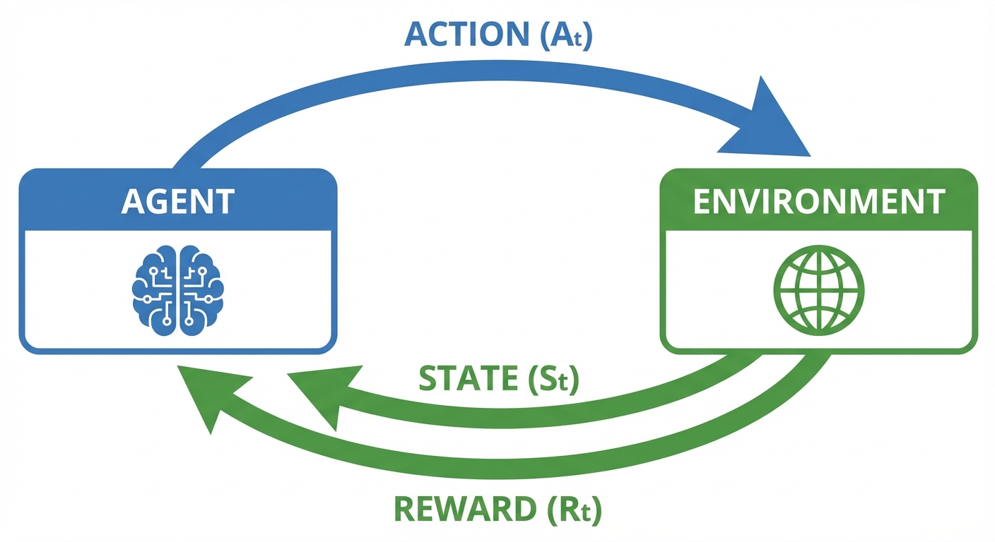
7. Introduction to Reinforcement Learning (RL)

RL addresses Sequential Decision Problems where an agent learns to make decisions by interacting with an environment, rather than planning with a complete model beforehand.

The RL Framework

• Agent: The learner and decision-maker.
• Environment: Everything the agent interacts with.
• Signal Exchange:
  1. Agent observes state .
  2. Agent performs action .
  3. Environment returns reward and next state .

Markov Decision Process (MDP)

RL problems are mathematically formalized as MDPs:

• Set of states .
• Set of actions .
• Transition function .
• Reward function .

Key Concepts

• Policy (): The agent's strategy. It maps states to actions ().
• Return: The objective is to maximize the expected cumulative reward (often discounted over time).
• Exploration vs. Exploitation: The dilemma between trying new actions to find better rewards (exploration) and using known actions to gain guaranteed rewards (exploitation).