Unit 5 - Notes
Unit 5: Ensemble Learning
1. Introduction to Ensemble Learning
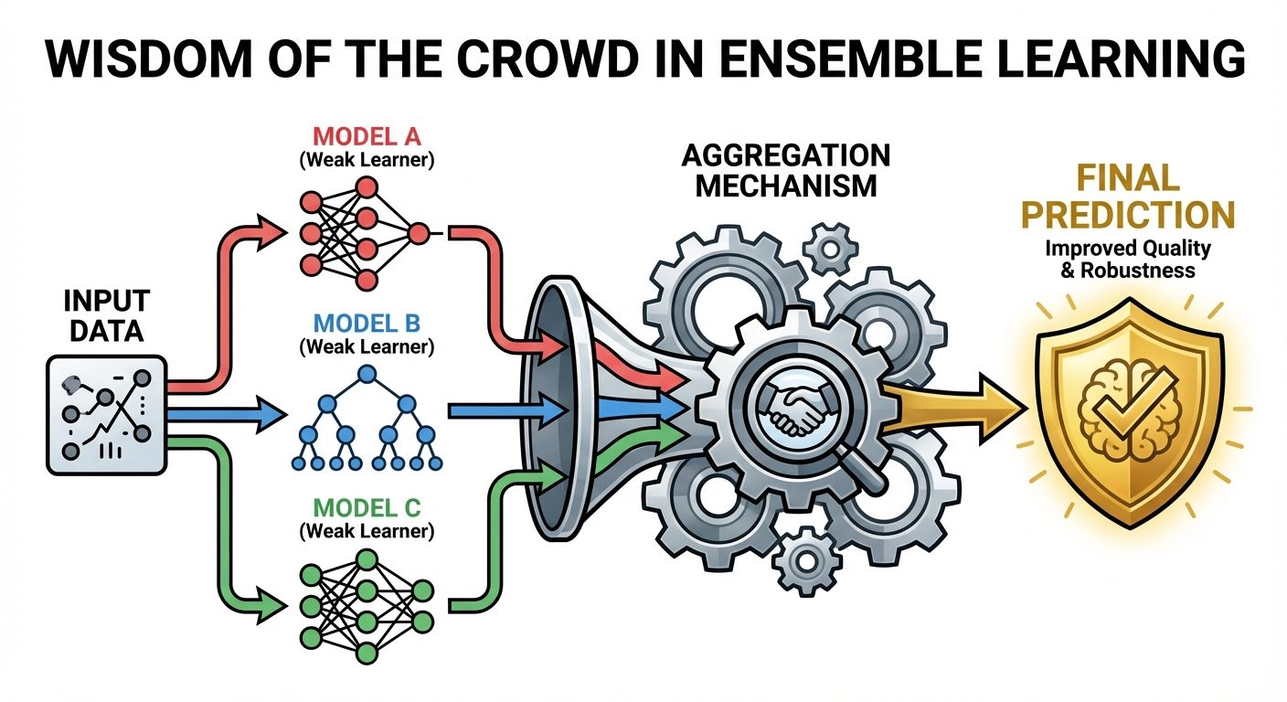
Ensemble Learning is a machine learning paradigm where multiple models (often called "weak learners" or "base estimators") are trained to solve the same problem and combined to get better results. The main hypothesis is that combining multiple models often produces a much stronger model than any single one of them.
Key Concepts
- Weak Learner: A model that performs slightly better than random guessing (e.g., a shallow decision tree or "stump").
- Strong Learner: A robust model with high accuracy and generalization capabilities, resulting from the ensemble process.
- Wisdom of the Crowd: If individual models have low correlation in their errors, averaging them cancels out random noise.
The Bias-Variance Tradeoff in Ensembles
- Bagging: Primarily reduces Variance (overfitting).
- Boosting: Primarily reduces Bias (underfitting) and variance.
2. Majority Voting Classifier
Majority voting is the simplest form of ensemble learning, typically used for classification problems.
Types of Voting
- Hard Voting:
- Each base model predicts a class label.
- The ensemble predicts the class that gets the most votes (mode).
- Example: Model A: Class 1, Model B: Class 1, Model C: Class 2. Final: Class 1.
- Soft Voting:
- Each base model predicts probabilities for each class.
- The ensemble averages the probabilities and picks the class with the highest average probability.
- Requirement: Base models must be calibrated (able to output
predict_proba).
Mathematical Formulation
Let be the classifiers.
For Hard Voting, predicted class is:
3. Bagging (Bootstrap Aggregating) Ensembles
Bagging is a parallel ensemble method designed to improve stability and accuracy.
The Algorithm
- Bootstrapping: Create subsets of the original training data by sampling with replacement. Some data points may appear multiple times in a subset, while others are omitted (Out-of-Bag).
- Parallel Training: Train a separate base model (usually a Decision Tree) on each subset independently.
- Aggregation:
- Classification: Majority Voting.
- Regression: Average the outputs.
Random Forest
Random Forest is the most popular implementation of Bagging. It adds an extra layer of randomness to standard bagging.
- Mechanism:
- Create bootstrap samples.
- Build a decision tree for each sample.
- Crucial Difference: At each node split, the algorithm selects a random subset of features (typically ) rather than evaluating all features.
- Benefits: This decorrelates the trees. If one feature is very strong, standard bagging would result in identical trees. Random Forest forces trees to use different features, increasing diversity.
- Out-of-Bag (OOB) Error: Data points not included in the bootstrap sample for a specific tree can be used as a validation set for that tree, removing the need for a separate validation set.
4. Boosting Ensembles
Boosting is a sequential ensemble method. Unlike Bagging, where models are independent, Boosting models depend on the previous ones.
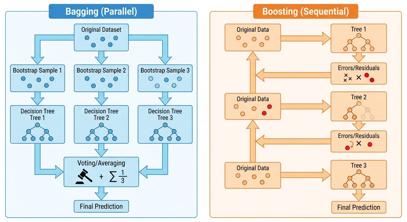
AdaBoost (Adaptive Boosting)
- Core Idea: Pay more attention to data points that were misclassified by the previous model.
- Process:
- Assign equal weights to all training samples.
- Train a weak learner (usually a decision stump—a tree with depth 1).
- Calculate error rate. Increase weights of misclassified instances; decrease weights of correctly classified ones.
- Train the next learner on the weighted data.
- Combine predictions using a weighted majority vote (better models get more say).
Gradient Boosting Machines (GBM)
- Core Idea: Instead of updating weights, train the new model to predict the residuals (errors) of the previous model.
- Process:
- Train a base model (e.g., predict the mean of the target).
- Calculate residuals: .
- Train a new tree to predict these residuals.
- Update the prediction: .
- Repeat.
- Gradient Descent: GBM optimizes a differentiable loss function. The residuals represent the negative gradient of the loss function.
5. Advanced Boosting Libraries
Modern machine learning competitions (like Kaggle) are often dominated by these three optimized implementations of Gradient Boosting.
XGBoost (eXtreme Gradient Boosting)
- Key Features:
- Regularization: Includes L1 (Lasso) and L2 (Ridge) regularization to prevent overfitting (standard GBM does not).
- Sparsity Awareness: Automatically handles missing values.
- Block Structure: Parallelizes tree construction (finding the best split).
- Tree Pruning: Uses "max_depth" parameter and prunes trees backwards.
LightGBM (Light Gradient Boosting Machine)
- Key Features:
- Leaf-wise Growth: Grows trees vertically (leaf-wise) rather than horizontally (level-wise). This results in deeper trees with lower loss but higher risk of overfitting (requires
max_depthlimit). - Histogram-based: Bins continuous feature values into discrete bins (histograms), speeding up split finding significantly.
- GOSS (Gradient-based One-Side Sampling): Keeps instances with large gradients (large errors) and randomly samples those with small gradients to speed up training.
- Leaf-wise Growth: Grows trees vertically (leaf-wise) rather than horizontally (level-wise). This results in deeper trees with lower loss but higher risk of overfitting (requires
CatBoost (Categorical Boosting)
- Key Features:
- Native Categorical Support: Handles categorical features automatically without One-Hot Encoding (uses Ordered Target Statistics).
- Ordered Boosting: Reduces prediction shift (a type of data leakage) by using a permutation-driven approach.
- Symmetric Trees: Builds balanced trees, which helps in execution speed (prediction time).
6. Ensemble Regression Models
While classifiers vote, regressors average.
- Voting Regressor: Averages the predictions of distinct algorithms (e.g., Linear Regression + SVR + Random Forest).
- Bagging Regressor: Averages predictions from multiple trees trained on bootstrap samples.
- Boosting Regressor: Starts with a constant (mean) and sequentially adds trees that predict the residual error. The final prediction is the sum of the constant and the weighted contributions of all trees.
7. Model Evaluation & Hyperparameter Tuning
Cross-Validation Strategies
To ensure the model generalizes well to unseen data.
- K-Fold Cross-Validation: Split data into folds. Train on , validate on 1. Repeat times. Average the score.
- Stratified K-Fold: Ensures each fold has the same proportion of class labels as the whole dataset (essential for imbalanced data).
- Time Series Split: For temporal data. Training set grows incrementally; validation set is always "future" data relative to training.
Pipelines
sklearn.pipeline.Pipeline chains preprocessing and modeling steps into a single object.
- Purpose: Prevents Data Leakage. Ensure scaling/imputation happens inside the cross-validation loop (fitted only on training fold, applied to validation fold).
- Structure:
Pipeline([('scaler', StandardScaler()), ('pca', PCA()), ('clf', RandomForestClassifier())])
Hyperparameter Tuning Techniques
Hyperparameters are settings external to the model (e.g., Tree Depth, Learning Rate) that must be set before training.
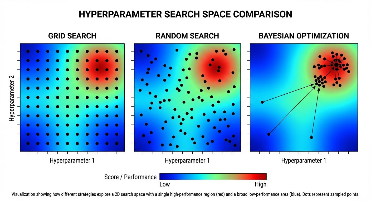
1. Grid Search
- Defines a grid of hyperparameter values.
- Exhaustively evaluates every combination.
- Pro: Guaranteed to find the best combination within the grid.
- Con: Computationally expensive; combinatorial explosion.
2. Random Search
- Defines a distribution for hyperparameters.
- Randomly samples a fixed number of combinations.
- Pro: Faster; more likely to find important parameters than Grid Search given the same compute budget.
3. Bayesian Optimization
- Builds a probabilistic model (Surrogate Model) of the objective function (Model performance vs. Hyperparameters).
- Uses past evaluation results to choose the next hyperparameter values to test.
- Balances Exploration (trying uncertain regions) and Exploitation (focusing on promising regions).
- Libraries:
Hyperopt,Optuna.
Summary Table: Tuning Methods
| Feature | Grid Search | Random Search | Bayesian Optimization |
|---|---|---|---|
| Search Strategy | Exhaustive | Stochastic (Random) | Informed (Probabilistic) |
| Computation | Very High | Moderate | Moderate/Low |
| Efficiency | Low | Medium | High |
| Best Use | Small parameter space | Large parameter space | Expensive model training |