Unit 4 - Notes
Unit 4: Regression
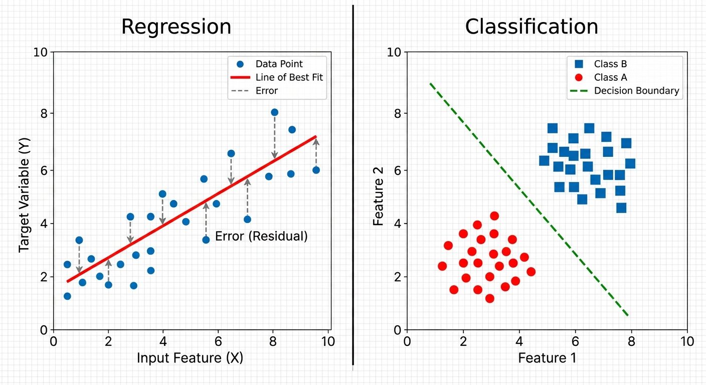
1. Regression vs. Classification
In supervised machine learning, the distinction between regression and classification lies in the nature of the target variable (output).
| Feature | Regression | Classification |
|---|---|---|
| Output Type | Continuous (numerical) values. | Categorical (discrete) class labels. |
| Goal | To predict a specific quantity (e.g., price, temperature, sales). | To predict group membership (e.g., spam/not spam, digit 0-9). |
| Evaluation Metrics | RMSE (Root Mean Squared Error), MAE (Mean Absolute Error), . | Accuracy, Precision, Recall, F1-Score, ROC-AUC. |
| Boundary | Fits a line, curve, or hyperplane through the data points. | Finds a decision boundary that separates data points into classes. |
Visualizing the Difference
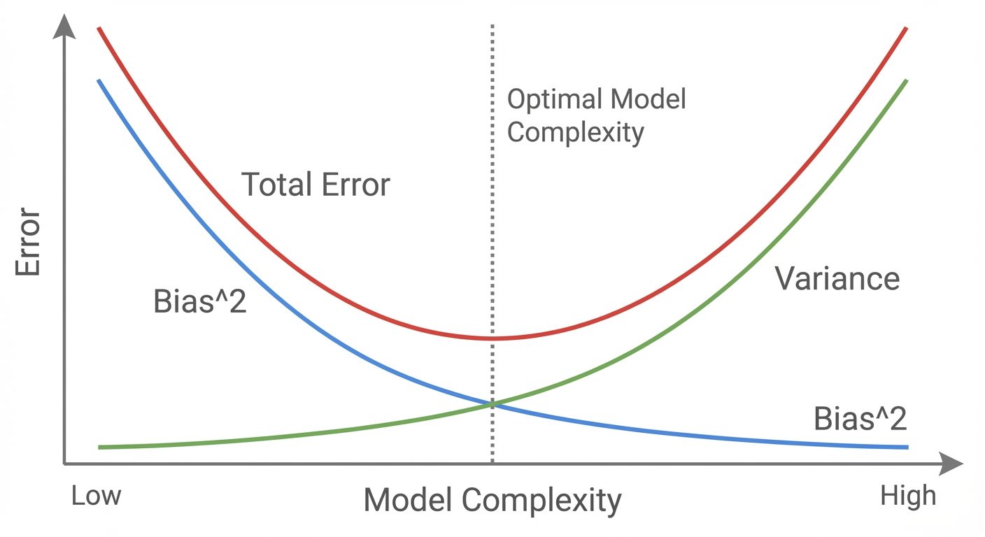
2. Bias-Variance Considerations in Regression
The bias-variance tradeoff is fundamental to understanding model generalization errors.
- Bias (Underfitting): Error introduced by approximating a real-world problem (which may be complex) by a much simpler model.
- High Bias: The model pays very little attention to the training data and oversimplifies the model. Example: Fitting a straight line to quadratic data.
- Variance (Overfitting): Error introduced by the model's sensitivity to small fluctuations in the training set.
- High Variance: The model pays too much attention to training data, capturing random noise rather than the underlying pattern. Example: High-degree polynomial passing through every data point.
Total Error Equation:
(Where is the irreducible error)
3. Simple Linear Regression (SLR)
SLR models the relationship between a single independent variable () and a dependent variable () using a straight line.
The Equation:
- : Intercept (value of when ).
- : Slope (rate of change).
- : Error term (residuals).
Cost Function (Ordinary Least Squares - OLS):
The goal is to minimize the Residual Sum of Squares (RSS):
Assumptions:
- Linearity: The relationship between and is linear.
- Independence: Observations are independent of each other.
- Homoscedasticity: The variance of residual is the same for any value of X.
- Normality: The error terms are normally distributed.
4. Multiple Linear Regression (MLR)
MLR extends SLR to include multiple independent variables ().
The Equation:
Matrix Form:
- The model fits a hyperplane in a -dimensional space rather than a line.
- Multicollinearity: A specific challenge in MLR where predictor variables are highly correlated with each other, making coefficient estimates unstable.
5. Interpretation of Coefficients
Interpreting values is crucial for inference.
- Intercept (): The expected value of when all predictors are zero. This may not always have a physical meaning depending on the data range.
- Slope Coefficients ():
- In SLR: A one-unit increase in is associated with a increase in .
- In MLR: A one-unit increase in is associated with a increase in , holding all other predictors constant.
Statistical Significance:
- p-value: Tests the null hypothesis that (no relationship). If , the predictor is statistically significant.
6. Polynomial Feature Expansion
When data shows a non-linear pattern (curved), linear regression can still be used by transforming the features. This is a form of Basis Expansion.
Concept:
Instead of fitting , we fit:
Although the relationship between and is non-linear, the model is still linear in parameters (), so OLS can still be used.
Implementation Example:
If input , a degree-2 polynomial expansion creates features: .
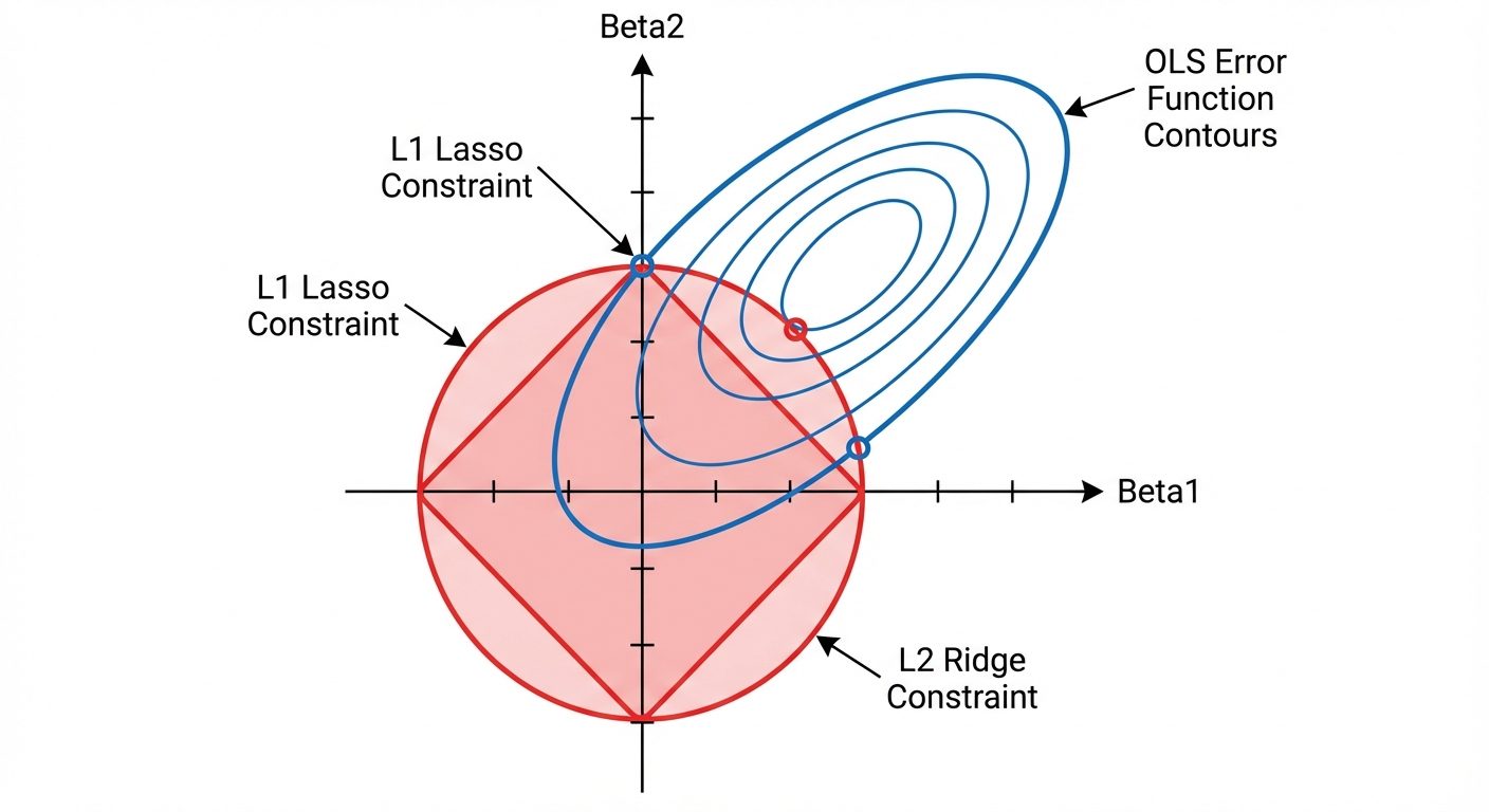
7. Regularized Regression Models
Regularization introduces a penalty term to the loss function to prevent overfitting by constraining the size of the coefficients.
A. Ridge Regression (L2 Regularization)
Adds a penalty equal to the square of the magnitude of coefficients.
- Effect: Shrinks coefficients toward zero but rarely exactly to zero.
- Use case: Good when many variables are correlated (handles multicollinearity).
B. Lasso Regression (L1 Regularization)
Adds a penalty equal to the absolute value of the magnitude of coefficients.
- Effect: Can shrink coefficients exactly to zero.
- Use case: Feature selection (produces sparse models).
C. Elastic Net
Combines L1 and L2 penalties.
8. Effect of Regularization on Model Complexity
The hyperparameter (lambda) controls the regularization strength.
- : Identical to OLS (No regularization).
- Small : Low Bias, High Variance. Model is flexible and can fit complex patterns.
- Large : High Bias, Low Variance. Coefficients are heavily penalized (shrunk). The model becomes very simple (flatter line).
- In Lasso, as , all coefficients become zero.
- In Ridge, as , all coefficients approach zero.
Selection: The optimal is usually selected via Cross-Validation.
9. Tree-Based Regression Models
Instead of a global linear equation, tree-based models partition the feature space into rectangular regions.
Decision Trees for Regression:
- Splitting: The algorithm recursively splits data based on feature values to minimize variance (usually MSE) within the resulting nodes.
- Leaf Value: The prediction for a new data point is the average (mean) value of the training samples falling into that leaf node.
Ensemble Methods:
- Random Forest: Builds many independent trees on bootstrapped data and averages their predictions (Bagging). Reduces variance.
- Gradient Boosting (e.g., XGBoost, LightGBM): Builds trees sequentially. Each new tree corrects the errors (residuals) made by the previous trees. Reduces bias and variance.
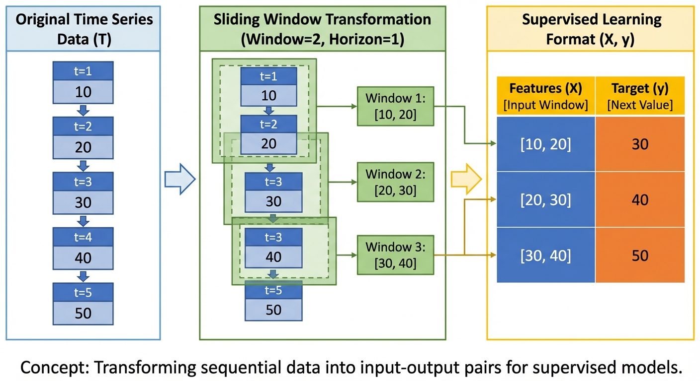
10. Time-Series Regression Models
Time-series regression involves predicting future values based on past history. The "independent variables" are often derived from the target variable itself.
Key Characteristics:
- Autocorrelation: Data points are not independent (today's price depends on yesterday's).
- Stationarity: Statistical properties (mean, variance) should ideally remain constant over time.
Feature Engineering for Time Series:
- Lag Features: Using as input to predict .
- Rolling Windows: Calculating moving averages or standard deviations over a window (e.g., past 7 days).
- Date-Time Features: Extracting components like Day of Week, Month, Quarter to capture seasonality.
Data Structure Transformation:
To use standard regression algorithms (like Linear Regression or Random Forest) on time series, the data must be transformed from a sequence to a supervised matrix.