Unit 6 - Notes
Unit 6: Unsupervised Learning
1. Introduction to Unsupervised Learning
Unsupervised learning is a branch of machine learning where the algorithm is trained on a dataset that is neither classified nor labeled. The algorithm essentially acts on the data without prior guidance.
Role of Unsupervised Learning
The primary goal is to model the underlying structure or distribution in the data in order to learn more about it.
- Pattern Discovery: Identifying hidden patterns or intrinsic structures in input data.
- Dimensionality Reduction: Compressing data while maintaining its structure and variance (e.g., PCA).
- Data Preprocessing: Used as a preliminary step for supervised learning to organize data.
Differences: Supervised vs. Unsupervised Learning
| Feature | Supervised Learning | Unsupervised Learning |
|---|---|---|
| Input Data | Labeled data (Input-Output pairs) | Unlabeled data (Input only) |
| Goal | Predict outcomes/classification | Find hidden structure/patterns |
| Feedback | Direct feedback (Correct/Incorrect) | No feedback loop |
| Complexity | Computationally simpler | Computationally complex |
| Algorithms | Regression, Decision Trees, SVM | K-Means, Apriori, PCA |
| Evaluation | Accuracy, Precision, Recall | Silhouette Score, Inertia, Davies-Bouldin |
2. Distance Metrics
In unsupervised learning (specifically clustering), "similarity" is often defined by the distance between data points.
Euclidean Distance
The straight-line distance between two points in Euclidean space. It is the most common metric.
- Formula:
- Use Case: General-purpose clustering when data is dense or continuous. Sensitive to outliers and scale (requires feature scaling).
Manhattan Distance ( Norm)
The sum of absolute differences between the coordinates of the points. Also known as "Taxicab geometry" (traveling along grid lines).
- Formula:
- Use Case: High-dimensional data where Euclidean distance becomes less distinguishing (Curse of Dimensionality).
Cosine Distance
Measures the cosine of the angle between two non-zero vectors. It measures orientation rather than magnitude.
- Formula:
- Use Case: Text analysis, document clustering, and recommendation systems where the magnitude (length of document) matters less than the content frequency (direction).
Choosing Appropriate Metrics
- Numeric/Geometric Data: Use Euclidean (standard) or Manhattan (high dimensions).
- Text/Sparse Data: Use Cosine distance.
- Categorical Data: Use Hamming distance or Jaccard index.
3. Partitioning Clustering Algorithms
Clustering is the task of dividing the population or data points into a number of groups such that data points in the same group are more similar to other data points in the same group than those in other groups.
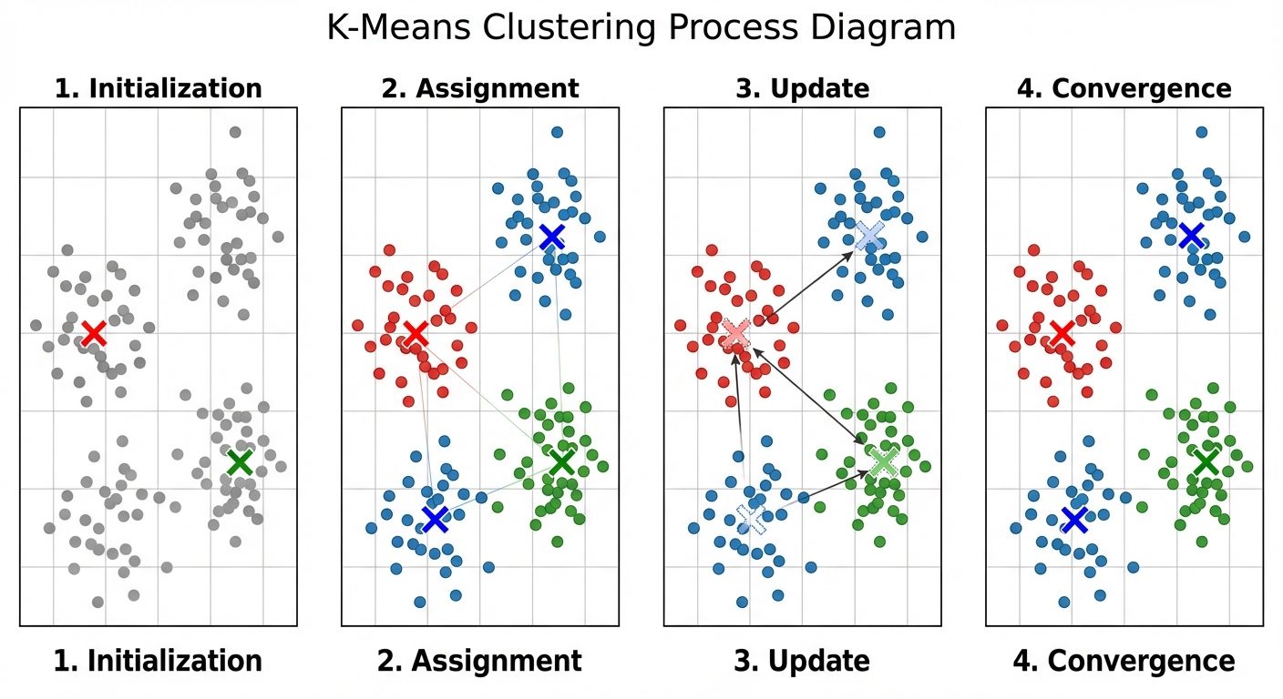
K-Means Clustering
An iterative algorithm that partitions the dataset into pre-defined distinct non-overlapping subgroups (clusters).
Algorithm Steps:
- Initialization: Choose random points as initial centroids.
- Assignment: Assign each data point to the nearest centroid (typically using Euclidean distance).
- Update: Calculate the new centroid of each cluster by taking the mean of all data points assigned to that cluster.
- Repeat: Repeat steps 2 and 3 until convergence (centroids do not change) or maximum iterations are reached.
The Elbow Method
A heuristic used to determine the optimal number of clusters ().
- Calculate the Within-Cluster Sum of Squares (WCSS) (also called Inertia) for a range of values (e.g., 1 to 10).
- Plot WCSS against .
- Select the value at the "elbow" point—the point where the rate of decrease shifts abruptly, indicating diminishing returns for adding more clusters.
K-Medoids (PAM - Partitioning Around Medoids)
Similar to K-Means, but instead of calculating the mean (centroid), it selects an actual data point from the cluster to represent it (the medoid).
- Comparison: K-Medoids is more robust to outliers than K-Means because outliers affect the mean significantly but have less impact on the median/medoid.
- Complexity: Higher computational cost than K-Means.
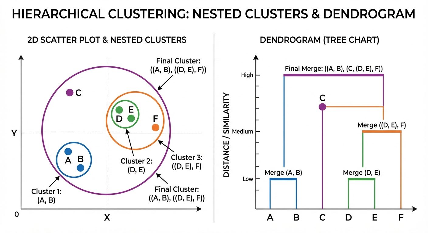
4. Hierarchical Clustering
Hierarchical clustering builds a hierarchy of clusters. It does not require specifying the number of clusters beforehand.
Types
- Agglomerative (Bottom-Up): Starts with each point as its own cluster. Pairs of clusters are merged as one moves up the hierarchy.
- Divisive (Top-Down): Starts with all points in one cluster. Splits are performed recursively as one moves down the hierarchy.
Dendrogram
A tree-like diagram that records the sequences of merges or splits. The height of the cut in the dendrogram determines the number of clusters.
Linkage Criteria
Determines the distance between two clusters:
- Single Linkage: Distance between the closest pair of points (creates long, chain-like clusters).
- Complete Linkage: Distance between the farthest pair of points (creates compact, spherical clusters).
- Average Linkage: Average distance between all pairs of points.
- Ward’s Method: Minimizes the variance within clusters being merged.
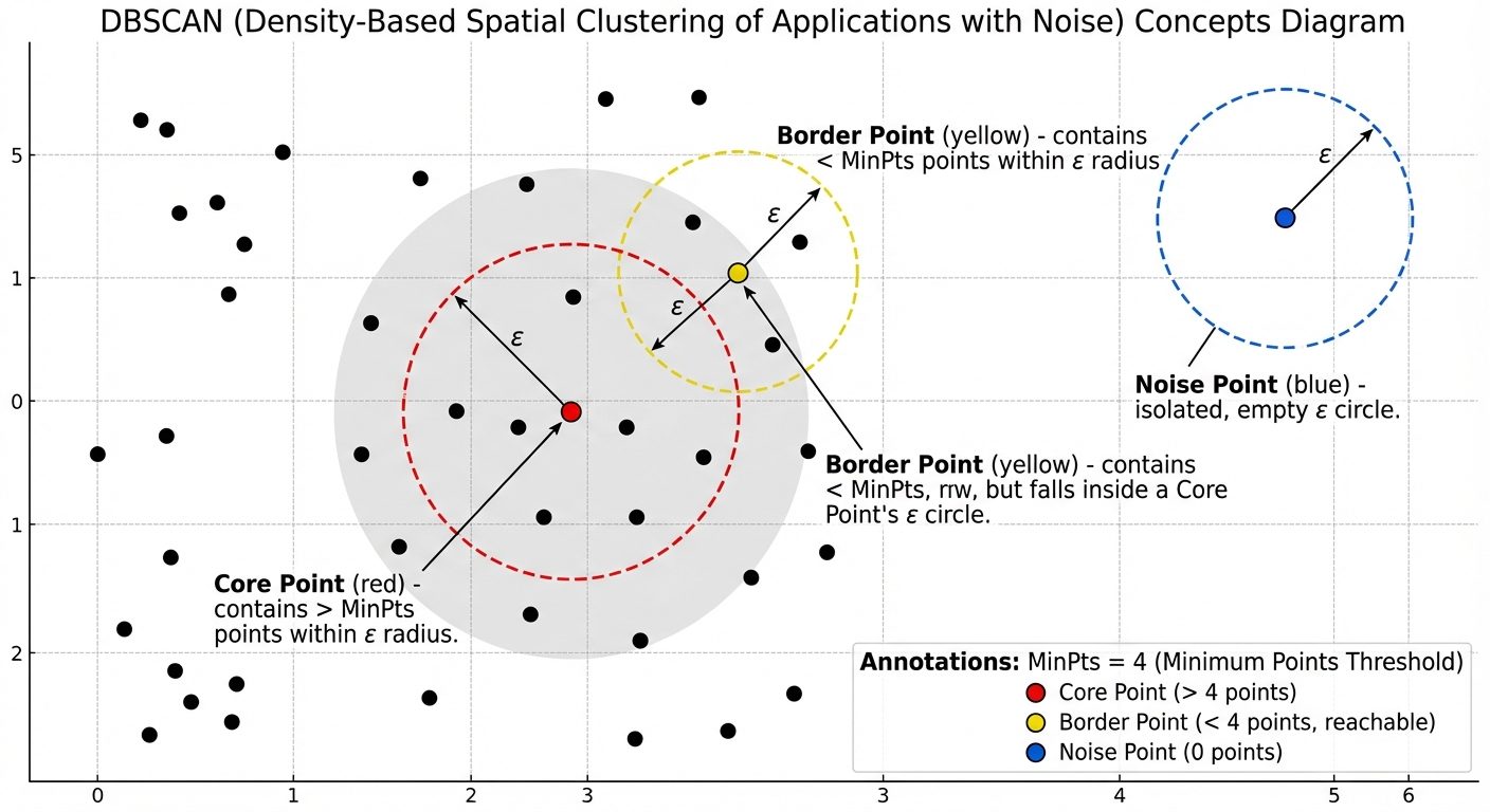
5. Density-Based Clustering (DBSCAN)
DBSCAN (Density-Based Spatial Clustering of Applications with Noise) groups together points that are close to each other (dense regions) and marks points that lie alone in low-density regions as outliers.
Key Concepts
- Epsilon (): The radius of the neighborhood around a data point.
- MinPts: The minimum number of data points required inside the -neighborhood to form a dense region.
Point Classifications
- Core Point: A point that has at least MinPts within its radius.
- Border Point: A point that has fewer than MinPts within its radius but is in the neighborhood of a Core Point.
- Noise Point (Outlier): A point that is neither a Core point nor a Border point.
Advantages:
- Can find arbitrarily shaped clusters (not just spherical like K-Means).
- Robust to outliers.
- Does not require specifying beforehand.
6. Anomaly Detection
Anomaly detection (Outlier Detection) identifies data points that deviate significantly from the majority of the data.
Relationship with Clustering
- Density-Based: Algorithms like DBSCAN explicitly label points in low-density regions as "Noise."
- Centroid-Based: In K-Means, points that are very far from their assigned centroid (high distance error) can be considered anomalies.
- Isolation Forest: An algorithm specifically designed for anomaly detection that isolates observations by randomly selecting a feature and then randomly selecting a split value.
7. Evaluating Clustering Algorithms
Since there are no "ground truth" labels in unsupervised learning, evaluation relies on internal validation metrics.
Inertia (Within-Cluster Sum of Squares)
- Calculates the sum of distances of all points within a cluster from the cluster centroid.
- Goal: Minimize Inertia.
- Limitation: Inertia keeps decreasing as the number of clusters increases (leads to overfitting if not checked via Elbow method).
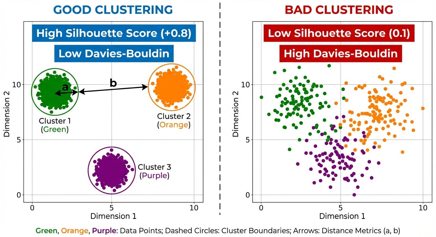
Silhouette Score
Measures how similar an object is to its own cluster (cohesion) compared to other clusters (separation).
- Formula:
- : Mean distance to other points in the same cluster.
- : Mean distance to points in the nearest neighboring cluster.
- Range: -1 to +1.
- +1: Highly dense cluster and well-separated from others.
- 0: Overlapping clusters.
- -1: Wrongly assigned points.
Davies-Bouldin Index
Ideally, clusters should be dense (low intra-cluster dispersion) and well-separated (high inter-cluster separation).
- It computes the ratio of within-cluster distances to between-cluster distances.
- Interpretation: Lower values indicate better clustering.