Unit 3 - Notes
Unit 3: Linear & Probabilistic Classification Models
1. Introduction to Supervised Learning
Supervised learning is a subcategory of machine learning and artificial intelligence where the algorithm is trained on input data that has been labeled for a particular output. The model learns a mapping function from input variables () to an output variable ().
- Goal: Approximate the mapping function so well that when you have new input data (), you can predict the output variables () for that data.
- Types of Supervised Learning:
- Classification: The output variable is a category (e.g., "Red" or "Blue", "Spam" or "Not Spam").
- Regression: The output variable is a real value (e.g., "Dollars", "Weight").
2. Linear Classification Models
Linear classifiers classify data by making a decision based on the value of a linear combination of the characteristics.
2.1 Perceptron
The Perceptron is the fundamental building block of artificial neural networks. It is a binary classification algorithm for supervised learning.
- Mechanism: It maps a real-valued vector input to a single binary output value (0 or 1).
- Mathematical Model:
Where:- : Weights representing the importance of inputs.
- : Bias term (shifts the activation function).
- Activation Function: Usually a Heaviside Step Function (returns 1 if , else 0).
- Limitations: The single-layer perceptron can only learn linearly separable patterns (it cannot solve XOR problems).
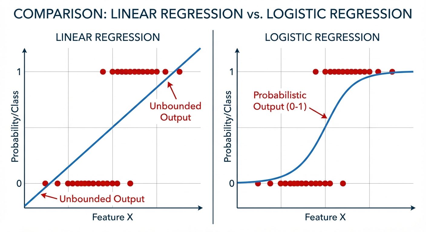
2.2 Logistic Regression
Despite its name, Logistic Regression is a classification algorithm, not a regression one. It is used to estimate discrete values (Binary values like 0/1, Yes/No) based on a given set of independent variables.
- Sigmoid Function: Instead of a raw linear output, the output is passed through a sigmoid function (logistic function) to map predictions to probabilities between 0 and 1.
- Decision Boundary: A threshold (usually 0.5) is set. If probability > 0.5, class is 1; otherwise, class is 0.
- Cost Function: Uses Log Loss (Cross-Entropy Loss) rather than Mean Squared Error to ensure convexity, allowing Gradient Descent to find the global minimum.
3. Probabilistic Classification Models
3.1 Naïve Bayes Classifier
Based on Bayes’ Theorem with an assumption of independence among predictors.
- Bayes' Theorem:
Where:- : Posterior probability (probability of class A given predictor B).
- : Likelihood.
- : Prior probability of class.
- : Prior probability of predictor.
- The "Naïve" Assumption: It assumes that the presence of a particular feature in a class is unrelated to the presence of any other feature (Conditional Independence). Even if features depend on each other, Naïve Bayes assumes they contribute independently to the probability.
- Types of Naïve Bayes:
- Gaussian: For continuous data following a normal distribution.
- Multinomial: For discrete counts (e.g., text classification/word counts).
- Bernoulli: For binary feature vectors.
4. Nonlinear & Distance-Based Models
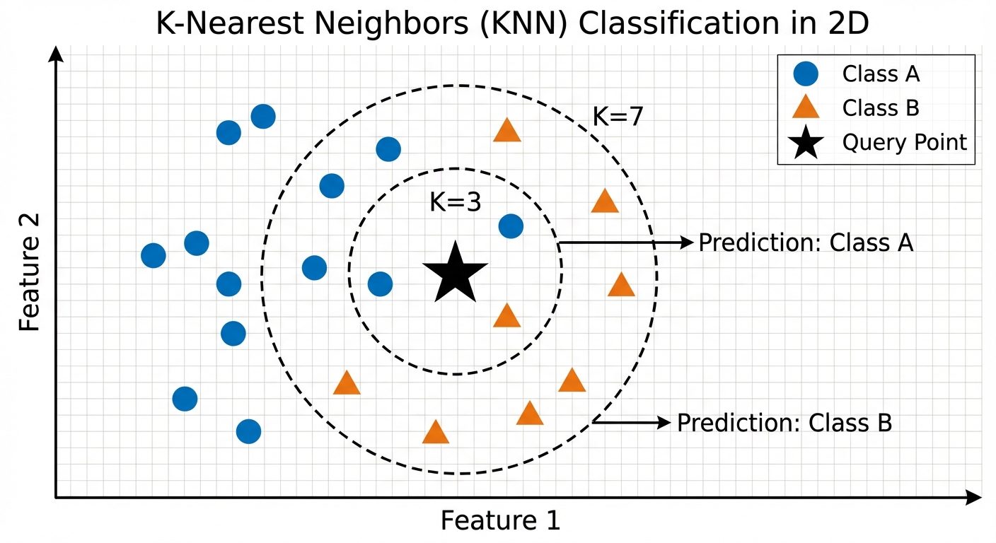
4.1 K-Nearest Neighbors (KNN)
KNN is a non-parametric, lazy learning algorithm. It makes no assumptions about the underlying data distribution.
- Logic: "Birds of a feather flock together." An object is classified by a plurality vote of its neighbors.
- The 'K' Factor: is the number of nearest neighbors to check.
- Small : Sensitive to noise (overfitting).
- Large : Smoother boundaries but may include points from other clusters (underfitting).
- Distance Metrics:
- Euclidean Distance (Straight line).
- Manhattan Distance (Grid-like path).
- Minkowski Distance.
4.2 Decision Tree
A tree-structured classifier where internal nodes represent the features of a dataset, branches represent the decision rules, and each leaf node represents the outcome.
- Structure:
- Root Node: The feature that best splits the data.
- Decision Node: Sub-nodes splitting further.
- Leaf Node: Final classification.
- Splitting Criteria:
- Entropy & Information Gain: Measures impurity. Higher entropy = more disorder. The goal is to maximize Information Gain (reduction in entropy).
- Gini Impurity: Measures the probability of misclassifying a randomly chosen element. Lower is better.
- Advantages: Easy to interpret visually; requires little data preprocessing.
- Disadvantages: Prone to overfitting (creating overly complex trees). Solved by pruning.
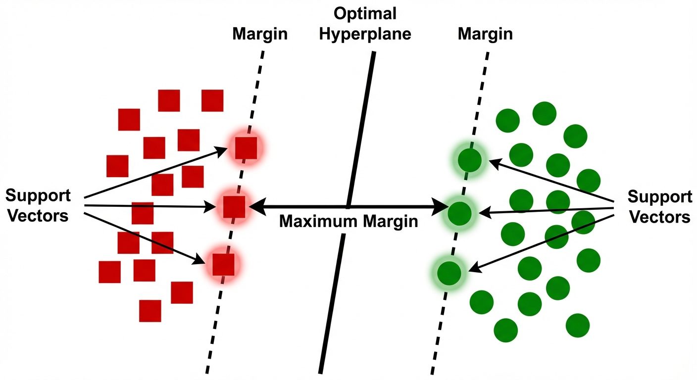
4.3 Support Vector Machine (SVM)
A powerful classifier that works by finding a hyperplane in an N-dimensional space that distinctly classifies the data points.
- Hyperplane: The decision boundary. In 2D, it's a line; in 3D, a plane.
- Support Vectors: Data points that are closer to the hyperplane and influence the position and orientation of the hyperplane.
- Margin: The distance between the hyperplane and the nearest data point from either class. SVM seeks to maximize this margin.
- Kernel Trick: If data is not linearly separable, SVM uses kernel functions (Linear, Polynomial, Radial Basis Function - RBF) to map data into a higher-dimensional space where it becomes separable.
5. Model Evaluation Metrics
Evaluating performance is critical to ensure the model generalizes well to unseen data.
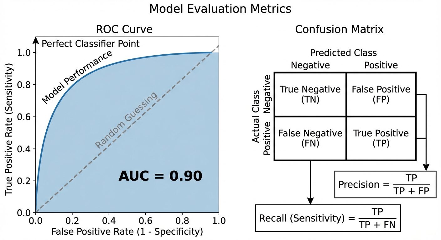
5.1 The Confusion Matrix
A table used to describe the performance of a classification model.
| Predicted Negative | Predicted Positive | |
|---|---|---|
| Actual Negative | True Negative (TN) | False Positive (FP) (Type I Error) |
| Actual Positive | False Negative (FN) (Type II Error) |
True Positive (TP) |
5.2 Basic Metrics
- Accuracy: Overall correctness. . (Misleading if classes are imbalanced).
- Precision: Out of all predicted positives, how many were actually positive?
Used when the cost of False Positives is high (e.g., Email Spam detection). - Recall (Sensitivity/TPR): Out of all actual positives, how many did we identify?
Used when the cost of False Negatives is high (e.g., Cancer detection). - F1-Score: Harmonic mean of Precision and Recall. Balances the two.
5.3 Advanced Evaluation: ROC & PR Curves
ROC Curve (Receiver Operating Characteristic)
A probability curve that plots the True Positive Rate (Recall) against the False Positive Rate (FPR) at various threshold settings.
- TPR (Y-axis): Sensitivity.
- FPR (X-axis): .
- Interpretation: Ideally, the curve hugs the top-left corner. A straight diagonal line represents random guessing.
ROC-AUC (Area Under The Curve)
- Represents the degree or measure of separability.
- AUC = 1.0: Perfect model.
- AUC = 0.5: No discriminative power (random guess).
- AUC = 0.0: Reciprocating the classes perfectly (predicting all negatives as positives and vice versa).
Precision-Recall (PR) Curve
Plots Precision (Y-axis) vs. Recall (X-axis).
- Usage: Unlike ROC, PR curves are better for imbalanced datasets (where the negative class dominates).
- Interpretation: A curve closer to the top-right corner indicates better performance.
AUC-PR
- The area under the Precision-Recall curve. High AUC-PR implies both low false positives and low false negatives.