Unit 2 - Notes
Unit 2: Feature Engineering and Dimensionality Reduction
1. Feature Selection Techniques
Feature selection involves selecting a subset of relevant features (variables, predictors) for use in model construction. It simplifies models, shortens training times, and reduces overfitting.
A. Filter Methods
Filter methods pick features based on statistical scores independent of the machine learning model.
1. Variance Threshold
This acts as a baseline feature selector. It removes all features whose variance doesn't meet some threshold. By default, it removes all zero-variance features (features that have the same value in all samples).
- Principle: If a feature has the same value for every single observation (Variance = 0), it provides no information to the model and can be discarded.
- Mathematical Concept: Variance () measures how far a set of numbers is spread out from their average value.
- Application:
- Boolean features: A Bernoulli random variable with probability has variance .
- If a feature is 0 or 1 in >99% of samples, it might be removed using a specific threshold.
2. Correlation-based Removal
This technique removes features that are highly correlated with each other (multicollinearity).
- Principle: If two features are highly correlated (e.g., Pearson correlation coefficient > 0.85), they provide redundant information. Keeping both increases computational cost and can make linear models unstable (high variance in coefficient estimates).
- Process:
- Calculate the correlation matrix for all features.
- Identify pairs of features with correlation above a defined threshold (absolute value).
- Drop one feature from each identified pair (usually the one with the lower correlation to the target variable).
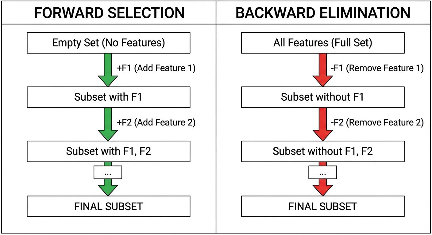
B. Wrapper Methods
Wrapper methods consider the selection of a set of features as a search problem, evaluating subsets based on model performance.
1. Forward Selection
An iterative, "greedy" method that starts with no features and adds them one by one.
- Steps:
- Start with a null model (no features).
- Train the model using each individual feature and calculate the performance (e.g., accuracy, RMSE).
- Select the feature that produces the best performance and add it to the model.
- Repeat the process, adding the next best feature that improves the model significantly.
- Stop when adding a new feature does not improve performance or a pre-set limit is reached.
2. Backward Elimination
The inverse of forward selection. It starts with all features and removes the least significant ones.
- Steps:
- Start with a model containing all features.
- Calculate the performance of the model.
- Iteratively remove the feature that contributes the least to the performance (or has the highest P-value in statistical tests).
- Retrain the model and measure performance.
- Stop when removing a feature significantly degrades model performance.
C. Embedded Methods
Embedded methods perform feature selection during the model training process itself.
1. Tree-based Feature Importance
Decision trees (and ensembles like Random Forest and Gradient Boosting) inherently rank features based on how well they improve the purity of the node.
- Gini Importance (or Mean Decrease Impurity): Measures the total reduction of the Gini impurity brought by that feature.
- Mechanism: Every time a node splits on a feature, the impurity (Gini or Entropy) decreases. The sum of these decreases across all trees in the forest is averaged for each feature. Features with higher sums are more important.
2. Feature Extraction and Engineering
Feature engineering is the art of transforming raw data into features that better represent the underlying problem to the predictive models.
A. Feature Extraction
Feature extraction creates new features from the original feature set, summarizing the information contained in the original features. Unlike selection, extraction changes the data values.
- Examples:
- Text: Converting text to vectors using TF-IDF or Word2Vec.
- Images: Using Convolutional Neural Networks (CNNs) to extract edges, textures, and shapes from raw pixels.
- Time Series: Extracting Fourier Transform components from wave data.
B. Creating New Features
Deriving new variables using domain knowledge or mathematical operations.
- Interaction Features: Combining two features to capture their joint effect.
- Example: In real estate, combining
LengthandWidthto createArea.
- Example: In real estate, combining
- Binning/Discretization: Converting continuous variables into categorical bins.
- Example: Converting
Age(0-100) intoAge_Group(Child, Adult, Senior).
- Example: Converting
- Date-Time Parsing: Extracting components like
Day_of_Week,Month, orIs_Weekendfrom a timestamp.
C. Aggregation Features
Common in transactional data or time-series data where one entity (e.g., a customer) has multiple rows.
- Operations:
Group Byentity ID followed by:Count: Number of transactions.Sum: Total money spent.Mean/Std Dev: Average transaction value and consistency.Min/Max: Range of activity.
3. Dimensionality Reduction Concepts
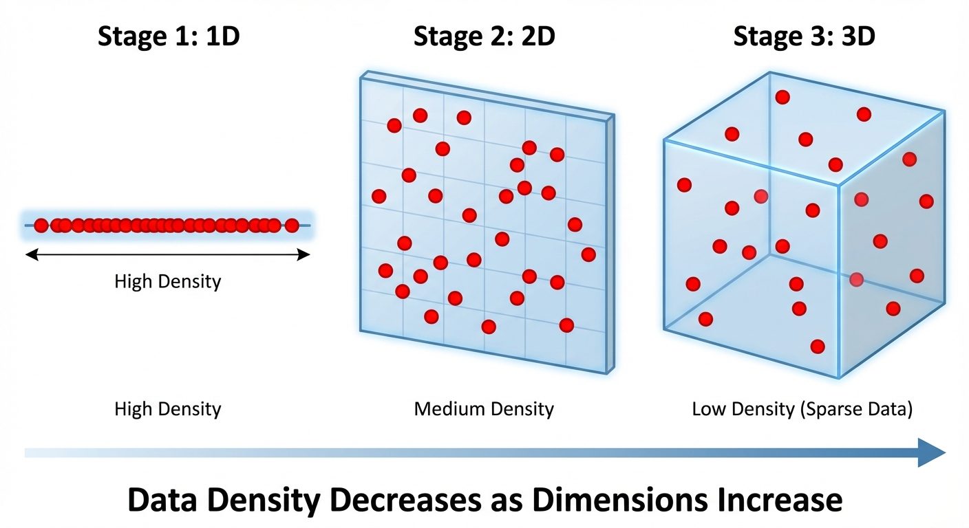
A. The Curse of Dimensionality
The "Curse of Dimensionality" refers to various phenomena that arise when analyzing data in high-dimensional spaces (hundreds or thousands of features) that do not occur in low-dimensional settings.
- Sparsity: As dimensions increase, the volume of the space increases exponentially. Data points become sparse, meaning the available data becomes insufficient to statistically represent the space.
- Distance Convergence: In very high dimensions, the Euclidean distance between the nearest and farthest data points becomes negligible. Distance-based algorithms (like K-Nearest Neighbors or K-Means) fail because "every point is far away from every other point."
- Overfitting: With too many features and fixed samples, models become complex and memorize noise rather than patterns.
B. Dimensionality Reduction
The process of reducing the number of random variables under consideration by obtaining a set of principal variables. It can be divided into feature selection and feature extraction (projection).
Goals:
- Visualization (reducing to 2D or 3D).
- Noise reduction.
- Improving computational efficiency.
- Mitigating the Curse of Dimensionality.
4. Linear Projection Methods
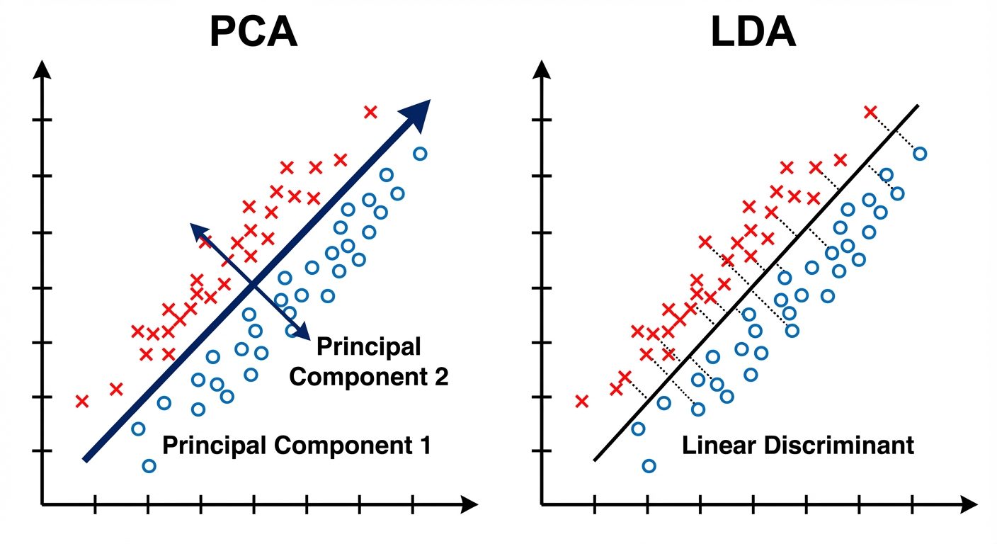
A. Principal Component Analysis (PCA)
PCA is an unsupervised linear transformation technique that reduces dimensionality while retaining as much variance (information) in the dataset as possible.
- Core Concept: PCA identifies new axes (Principal Components) that are orthogonal (perpendicular) to each other and aligned with the directions of maximum variance in the data.
- The Algorithm:
- Standardize the data (Mean = 0, Variance = 1).
- Compute the Covariance Matrix to identify correlations.
- Compute Eigenvectors and Eigenvalues of the covariance matrix.
- Eigenvectors point in the direction of the new axes.
- Eigenvalues represent the magnitude of variance in that direction.
- Sort Eigenvalues in descending order and select the top Eigenvectors.
- Project the original data onto this new -dimensional subspace.
Explained Variance Ratio
This metric tells us how much information (variance) can be attributed to each of the principal components.
- Usage: It is used to decide how many components to keep.
- Scree Plot: A graph plotting the explained variance ratio against the component index. One looks for an "elbow" in the plot where the marginal gain of adding a new component drops significantly.
- Example: "PC1 explains 60% of variance, PC2 explains 25%. Together they preserve 85% of the dataset's information."
B. Linear Discriminant Analysis (LDA)
LDA is a supervised dimensionality reduction technique. While PCA focuses on variance, LDA focuses on class separability.
- Goal: To project a dataset onto a lower-dimensional space with good class-separability in order to avoid overfitting ("curse of dimensionality") and also reduce computational costs.
- Mechanism: LDA finds a linear combination of features that characterizes or separates two or more classes of objects or events.
- Optimization Criterion: It maximizes the ratio of Between-Class Variance () to Within-Class Variance ().
- Between-Class Variance: Distance between the means of different classes (we want this large).
- Within-Class Variance: Spread of data around the mean of its own class (we want this small/tight).
Comparison: PCA vs. LDA
| Feature | PCA | LDA |
|---|---|---|
| Type | Unsupervised (ignores labels) | Supervised (uses class labels) |
| Objective | Maximize Variance | Maximize Class Separation |
| Components | Principal Components | Linear Discriminants |
| Use Case | Visualization, Noise Reduction, General Feature reduction | Classification pre-processing |