Unit 1 - Notes
Unit 1: Data Pre-processing
1. Introduction to Data and Pre-processing
Data Pre-processing is a data mining technique that involves transforming raw data into an understandable format. Real-world data is often incomplete, inconsistent, and lacking in certain behaviors or trends, and is likely to contain many errors. Pre-processing is a proven method of resolving such issues.
The "Garbage In, Garbage Out" (GIGO) Principle:
If the input data is of poor quality, the output of the machine learning model will be of poor quality, regardless of how sophisticated the algorithm is.
Key Steps in Pre-processing Pipeline:
- Data Cleaning: Handling missing data, noisy data, etc.
- Data Integration: Combining data from multiple sources.
- Data Reduction: Dimensionality reduction, numerosity reduction.
- Data Transformation: Normalization, discretization, hierarchy generation.
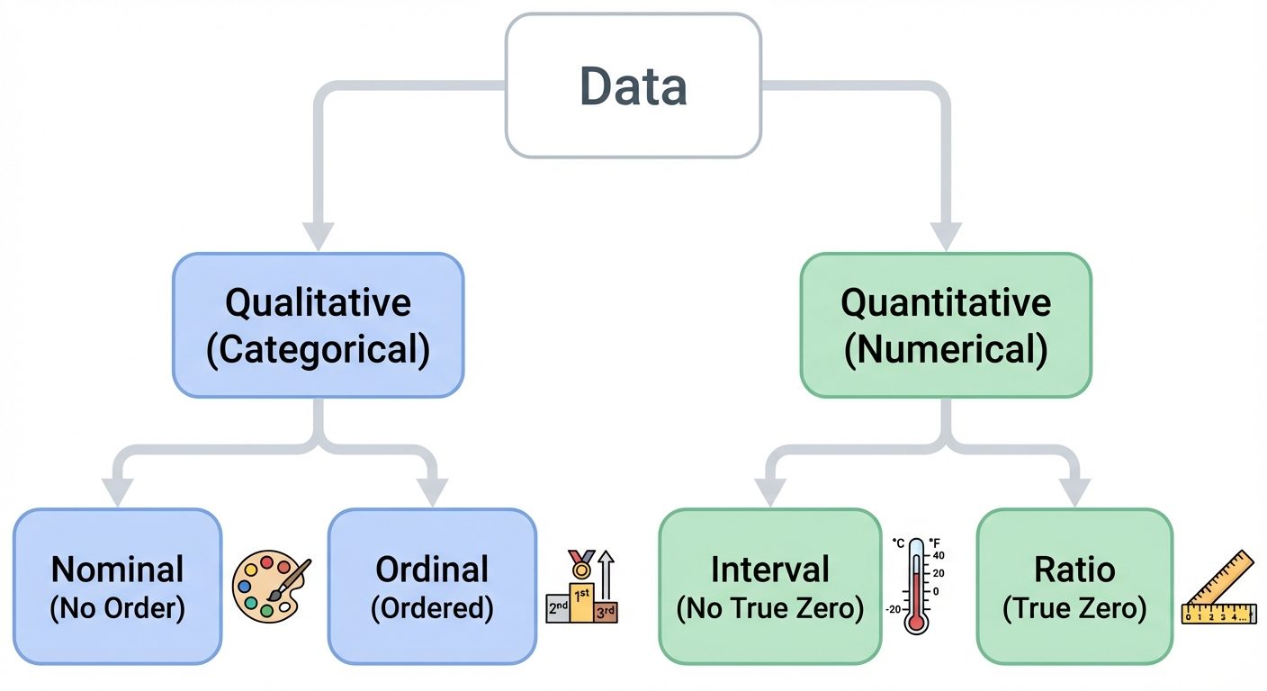
2. Types of Data
Understanding the data type is crucial for selecting the correct visualization techniques and machine learning algorithms.
A. Qualitative (Categorical) Data
Data that describes characteristics or qualities. It cannot be counted or measured in the traditional sense.
- Nominal Data:
- Categories without any intrinsic ordering.
- Examples: Gender (Male/Female), Color (Red/Blue/Green), Zip Codes.
- Statistical limit: Mode.
- Ordinal Data:
- Categories with a clear ordering or ranking.
- Examples: Education Level (High School < Bachelor's < Master's), Customer Satisfaction (Low < Medium < High).
- Statistical limit: Median, Percentiles.
B. Quantitative (Numerical) Data
Data that deals with numbers and things you can measure objectively.
- Interval Data:
- Numeric scales where we know the order and the exact difference between values.
- Key characteristic: No true zero point (0 does not mean "nothing").
- Examples: Temperature in Celsius (0°C is not "no temperature"), pH scale.
- Operations: Addition/Subtraction allowed; Multiplication/Division not meaningful.
- Ratio Data:
- Numeric scales with a clear definition of zero.
- Key characteristic: True zero point exists.
- Examples: Height, Weight, Salary, Age.
- Operations: All arithmetic operations allowed (e.g., A is twice as heavy as B).
C. Structured vs. Unstructured
- Structured: Highly organized (SQL tables, CSVs).
- Unstructured: No pre-defined model (Text, Images, Audio, Video).
- Semi-Structured: JSON, XML (contains tags/markers).
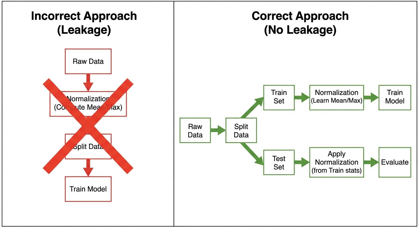
3. The Concept of Data Leakage
Data Leakage occurs when information from outside the training dataset is used to create the model. This allows the model to "see" the unexpected data or the test data during training, leading to overly optimistic performance scores that drop significantly on real-world data.
Common Causes:
- Leaking Test Data into Training Data: Performing pre-processing (like imputation or scaling) on the entire dataset before splitting into train/test sets.
- Leaking Future Information: Including features that would not be available at the time of prediction (e.g., using "Time_to_Churn" to predict "Will_Churn").
Prevention:
- Split First, Process Later: Always split data into Train/Test sets before any transformation.
- Pipelines: Use
sklearn.pipeline.Pipelineto ensure transformations fit only on training data and transform the test data using those learned parameters.
4. Handling Missing Values
Missing data is marked as NaN (Not a Number), null, or specific placeholders like -999.
Mechanisms of Missingness:
- MCAR (Missing Completely at Random): Probability of missingness is unrelated to any data.
- MAR (Missing at Random): Missingness is related to observed data (e.g., men might be less likely to report depression than women, but within the "men" group, it is random).
- MNAR (Missing Not at Random): Missingness depends on the missing value itself (e.g., rich people not disclosing income).
Handling Techniques:
1. Deletion
- Listwise Deletion: Drop entire rows with nulls. (Risk: Loss of data).
- Pairwise Deletion: Only analyze cases with available data for specific variables.
2. Imputation (Simple)
- Mean/Median: Good for numerical data. Median is robust to outliers.
- Mode: Used for categorical data.
- Constant: Fill with 0 or "Unknown".
3. Imputation (Advanced)
- KNN Imputation: Find nearest neighbors and use their average to fill the gap.
- Multivariate Imputation by Chained Equations (MICE): Models each feature with missing values as a function of other features.
# Python Example using Scikit-Learn
from sklearn.impute import SimpleImputer
import numpy as np

# Mean Imputation
imputer = SimpleImputer(missing_values=np.nan, strategy='mean')
X_train_imputed = imputer.fit_transform(X_train)
5. Outlier Handling
Outliers are data points that differ significantly from other observations. They can skew statistical measures and ruin the performance of distance-based algorithms (like KNN or SVM) and linear models.
Detection Methods:
- Z-Score: measures how many standard deviations a point is from the mean.
- Rule: If , it is an outlier.
- Assumption: Data follows a Gaussian (Normal) distribution.
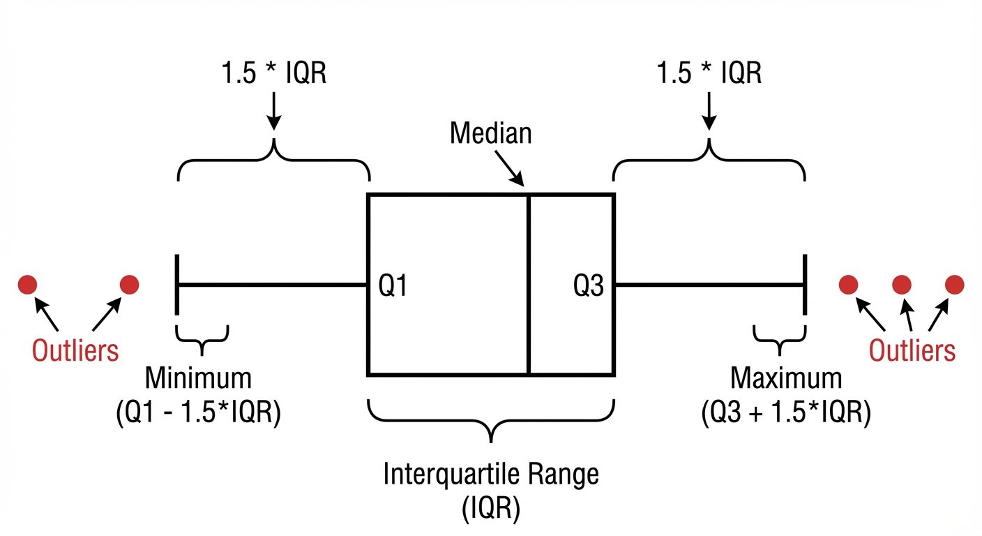
- IQR (Interquartile Range) Method: Robust to non-normal distributions.
- Lower Bound:
- Upper Bound:
Treatment Methods:
- Trimming: Remove the outliers.
- Capping (Winsorizing): Replace outliers with the upper/lower bound values.
- Transformation: Log transformation or Box-Cox transformation to reduce the impact of extreme values.
6. Handling Categorical Data
Machine Learning models require numerical input. Categorical text data must be converted.
1. One-Hot Encoding (Nominal Data)
Creates a new binary column for each unique category.
- Example: Color (Red, Blue) Is_Red (1,0), Is_Blue (0,1).
- Pros: No order implied.
- Cons: Curse of dimensionality (if cardinality is high).
- Dummy Variable Trap: Multicollinearity introduced if columns are created for categories. usually drop one column ().
2. Label Encoding (Ordinal Data)
Assigns an integer to each category based on alphabetical order or rank.
- Example: Low=0, Medium=1, High=2.
- Pros: Preserves order.
- Cons: If used on nominal data, the model might learn false relationships (e.g., Blue(2) > Red(1)).
3. Frequency/Count Encoding
Replace category with the count of its occurrences in the train set.
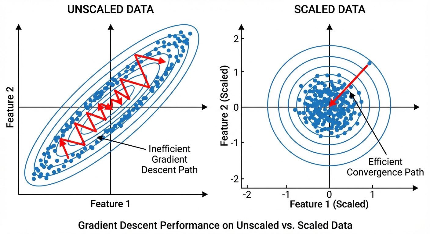
7. Scaling and Normalization
Feature scaling ensures that all features contribute equally to the result. Without scaling, a feature with a range [0, 10000] (e.g., Salary) will dominate a feature with range [0, 1] (e.g., Age/100) in distance calculations.
A. Standardization (Z-Score Normalization)
Rescales data to have a mean () of 0 and standard deviation () of 1.
- Best for: SVM, Logistic Regression, Neural Networks.
- Properties: Preserves outliers (doesn't cap them).
B. Normalization (Min-Max Scaling)
Rescales data to a fixed range, usually [0, 1].
- Best for: Neural Networks, Image Processing, algorithms requiring bounded input.
- Properties: Highly sensitive to outliers.
| Feature | Standardization | Normalization |
|---|---|---|
| Range | Unbounded | [0, 1] |
| Outliers | Robust | Sensitive |
| Distribution | Gaussian (Bell Curve) | Non-Gaussian |
8. Class Imbalance Handling
Occurs when the target class has an uneven distribution of observations (e.g., Fraud Detection: 99% Normal, 1% Fraud). Models tend to be biased toward the majority class.
Techniques:
1. Resampling
- Random Undersampling: Removing examples from the majority class.
- Issue: Loss of potentially valuable information.
- Random Oversampling: Duplicating examples from the minority class.
- Issue: Overfitting (model memorizes duplicates).
2. SMOTE (Synthetic Minority Over-sampling Technique)
Instead of duplicating, SMOTE creates synthetic new data points.
- Select a minority sample .
- Find its nearest neighbors (e.g., ).
- Draw a line between and .
- Generate a new point randomly somewhere on that line.
3. Algorithmic Approaches
- Class Weights: Modify the loss function to penalize the model more heavily for misclassifying the minority class (e.g.,
class_weight='balanced'in sklearn). - Tree-based models: Random Forests and XGBoost are generally more robust to imbalance than linear models.
# SMOTE Example
from imblearn.over_sampling import SMOTE
X_resampled, y_resampled = SMOTE().fit_resample(X_train, y_train)