Unit 5: Statistics for ML

1. Statistical Foundations for Machine Learning

Machine learning relies heavily on statistics to draw inferences from data. Understanding the relationship between data samples and the underlying population is crucial for building generalized models.

1.1 Sampling and Population

• Population (): The entire pool from which a statistical sample is drawn. It represents every possible observation of a specific phenomenon (e.g., all humans on Earth).
• Sample (): A subset of the population used to represent the whole group.
• Sampling: The process of selecting observations from the population.
  • Goal: To obtain a representative sample that minimizes bias, allowing the ML model to generalize well to unseen data.
  • Bias: Systematic error introduced if the sample does not accurately represent the population (e.g., training a face recognition model only on one ethnicity).

1.2 Hypothesis Testing

A formal procedure for investigating our ideas about the world using statistics. In ML, this is often used for feature selection or model comparison.

• Null Hypothesis (): The default assumption (e.g., "There is no difference between Model A and Model B").
• Alternative Hypothesis (): The theory we want to prove (e.g., "Model A performs better than Model B").
• P-value: The probability of observing the results assuming is true.
  • Low p-value (): Reject (Statistically Significant).
  • High p-value: Fail to reject .
• Type I Error (False Positive): Rejecting when it is actually true.
• Type II Error (False Negative): Failing to reject when it is actually false.

1.3 Confidence Intervals (CI)

A range of values derived from sample statistics that is likely to contain the value of an unknown population parameter.

• Formula:
  • : Sample mean
  • : Z-score (confidence level, e.g., 1.96 for 95%)
  • : Standard deviation
  • : Sample size
• Relevance in ML: Used to express uncertainty in model performance metrics (e.g., "Accuracy is 85% 2%").

1.4 Correlation

Measures the statistical relationship between two variables.

• Pearson Correlation Coefficient (): Measures linear correlation.
  • Range: .
  • : Perfect positive correlation.
  • : Perfect negative correlation.
  • : No linear correlation.
• Note: "Correlation does not imply causation." Two variables might be correlated due to a third confounding variable.

2. Estimation and Loss Functions

2.1 Maximum Likelihood Estimation (MLE)

MLE is a method to estimate the parameters () of a probability distribution or model by maximizing a likelihood function, so that the observed data is most probable.

• Likelihood Function : Measures the goodness of fit of a statistical model to a sample of data for given values of unknown parameters.
• Log-Likelihood: We usually work with the natural logarithm of the likelihood because:
  1. Probabilities are small; multiplying them leads to underflow. Summing logs is numerically stable.
  2. The maximum of the log function occurs at the same point as the original function.
• Goal:

2.2 Loss Functions (Cost Functions)

A loss function measures the difference between the predicted output () and the actual target (). The goal of training is to minimize this function.

• Mean Squared Error (MSE): Used for Regression.
  
  • Penalizes large errors heavily (due to squaring).
• Cross-Entropy Loss (Log Loss): Used for Classification.
  
  • Penalizes confident but wrong predictions heavily.

3. The Optimization Landscape

Understanding the geometry of the loss function is vital for training models effectively.

3.1 Convex vs. Non-convex Functions

• Convex Function:
  • Has only one minimum (Global Minimum).
  • Visual: A simple bowl shape.
  • Example: Linear Regression (MSE).
  • Benefit: Gradient Descent is guaranteed to converge to the global optimum.
• Non-convex Function:
  • Has multiple peaks and valleys.
  • Visual: A rugged mountain range.
  • Example: Deep Neural Networks.
  • Challenge: Optimization may get stuck in a suboptimal spot.

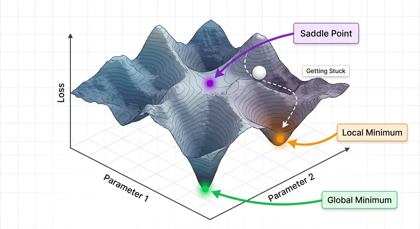
3.2 Minima and Saddle Points

• Global Minimum: The absolute lowest point in the entire loss landscape. This is the ideal model state.
• Local Minimum: A point lower than its immediate neighbors but higher than the global minimum. Algorithms can get "trapped" here.
• Saddle Points: Points where the gradient is zero (flat), but it is a minimum in one dimension and a maximum in another. These are common in high-dimensional spaces and slow down training.

4. Optimization Algorithms

Optimization algorithms update the model parameters to minimize the loss function.

4.1 Gradient Descent (GD)

An iterative optimization algorithm for finding the minimum of a function. It moves in the direction of the steepest descent (negative gradient).

• The Update Rule:
  
  • : Parameters (weights).
  • (Eta): Learning Rate.
  • : Gradient (slope) of the loss function.

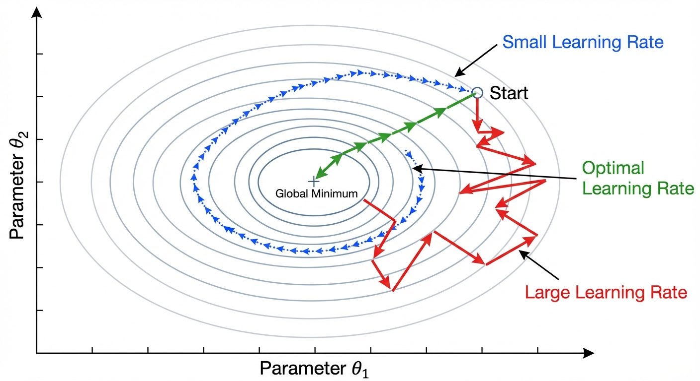
4.2 The Learning Rate ()

The hyperparameter that controls the step size at each iteration.

• Too Small: Convergence is very slow; the model may take forever to train.
• Too Large: The model may overshoot the minimum, fail to converge, or diverge (loss increases to infinity).
• Optimal: Converges quickly and smoothly.

4.3 Variants of Gradient Descent

1. Batch Gradient Descent:
   • Computes the gradient using the entire dataset.
   • Pros: Stable, guaranteed convergence for convex functions.
   • Cons: Very slow for large datasets; requires high memory.
2. Stochastic Gradient Descent (SGD):
   • Computes the gradient using a single training example chosen at random.
   • Pros: Faster per iteration; adds noise which helps escape local minima.
   • Cons: High variance updates; the cost function fluctuates heavily (noisy convergence).
3. Mini-Batch Gradient Descent:
   • Computes gradient using a small batch (e.g., 32, 64 samples).
   • Verdict: The standard compromise. Balances speed and stability.

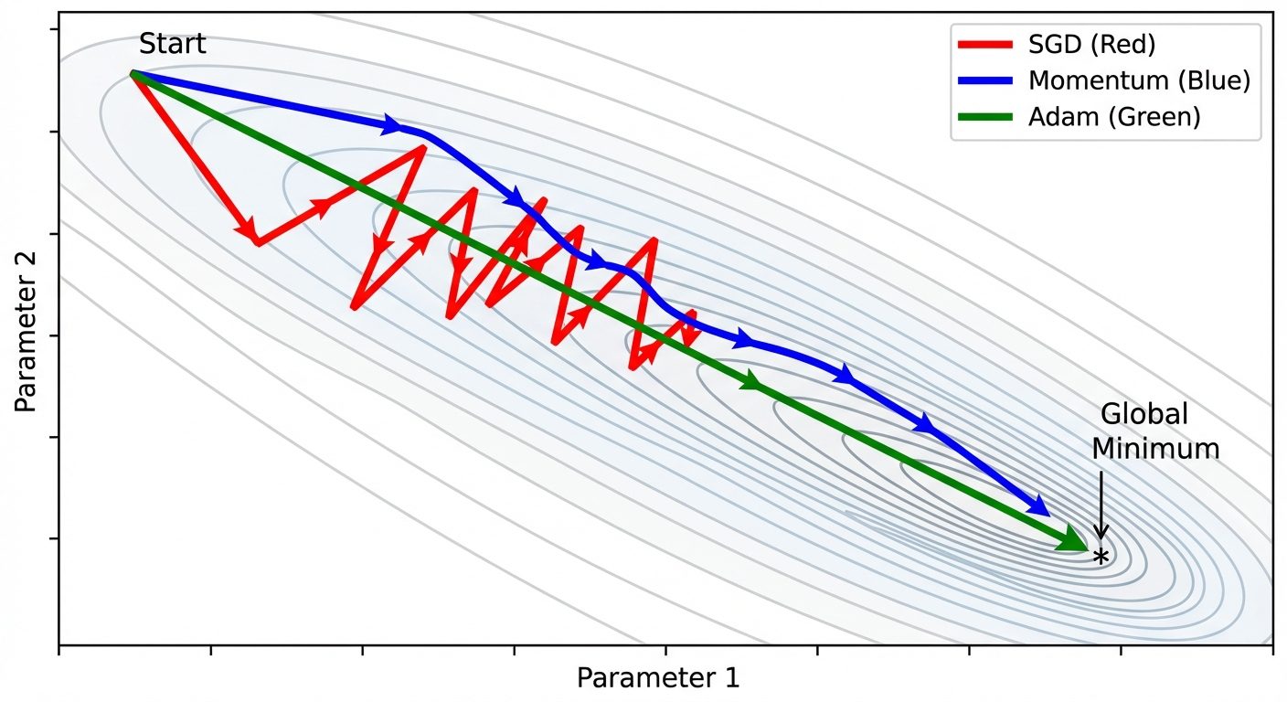
5. Advanced Optimizers

Standard SGD has trouble navigating "ravines" (areas where the surface curves much more steeply in one dimension than in another) and saddle points. Advanced optimizers address this using adaptive techniques.

5.1 Momentum

Momentum accelerates SGD in the relevant direction and dampens oscillations.

• Concept: It simulates a heavy ball rolling down a hill. It builds up velocity in directions with consistent gradients.
• Mechanism: It adds a fraction () of the previous update vector to the current update.
  
  
  
• Benefit: Helps plow through small local minima and saddle points; reduces oscillation in ravines.

5.2 RMSProp (Root Mean Square Propagation)

Addresses the issue of vanishing or exploding gradients by adapting the learning rate for each parameter individually.

• Mechanism: It maintains a moving average of the squared gradients. It divides the learning rate by the square root of this average.
• Effect:
  • Parameters with large gradients (steep slopes) get a reduced learning rate (prevents oscillations).
  • Parameters with small gradients (flat regions) get an increased learning rate (speeds up learning).

5.3 Adam (Adaptive Moment Estimation)

Currently the most popular optimizer. It combines the best properties of Momentum and RMSProp.

• Idea:
  1. Keeps track of an exponentially decaying average of past gradients (Momentum - first moment).
  2. Keeps track of an exponentially decaying average of past squared gradients (RMSProp - second moment).
• Bias Correction: Adam includes bias correction terms to account for initialization at zero.
• Why use Adam? It works well with default hyperparameters, handles sparse gradients, and converges fast.