Unit 4: Linear Algebra and Calculus

1. Linear Algebra Fundamentals

Linear algebra is the branch of mathematics concerning linear equations and linear maps. It is the language of data in Machine Learning (ML), defining how data is represented and manipulated.

1.1 Data Structures

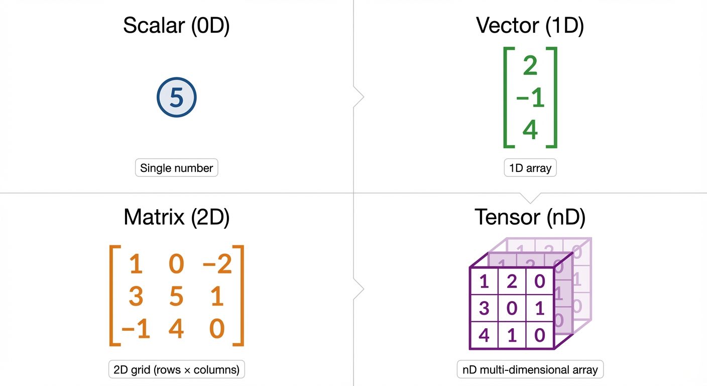
Data in ML is typically represented using the following structures:

• Scalars (Rank-0 Tensor):

  • A single numerical value.
  • Notation: Italic lower case letter (e.g., ).
  • Example: (representing a learning rate or a loss value).

• Vectors (Rank-1 Tensor):

  • An array of numbers (elements) arranged in an order. It represents a point in space with magnitude and direction.
  • Notation: Bold lower case letter (e.g., ).
  • Example: A single data point representing a house feature set: .

• Matrices (Rank-2 Tensor):

  • A 2-D array of numbers arranged in rows and columns.
  • Notation: Bold upper case letter (e.g., ).
  • Example: A dataset where rows are samples and columns are features. ( rows, columns).

• Tensors (Rank-n Tensor):

  • An array of numbers arranged on a regular grid with a variable number of axes.
  • Notation: Calligraphic letter (e.g., ).
  • Example: An image dataset input for a Convolutional Neural Network (Batch size Height Width Color Channels).

1.2 Eigenvalues and Eigenvectors

These concepts are critical for dimensionality reduction techniques like Principal Component Analysis (PCA).

• Definition: For a square matrix , an eigenvector is a non-zero vector that, when multiplied by , only changes in scale, not direction. The scaling factor is the eigenvalue .
• Equation:
  
• Interpretation:
  • Eigenvector (): Represents a direction of the transformation that remains invariant (doesn't rotate).
  • Eigenvalue (): Represents the magnitude of the stretch or shrink along the eigenvector's direction.

2. Probability Foundations

Probability theory provides a framework for managing uncertainty in Machine Learning models.

2.1 Random Variables

A random variable is a variable whose values depend on outcomes of a random phenomenon.

• Discrete Random Variables: Can take on a countable number of distinct values (e.g., Rolling a die: ). Described by a Probability Mass Function (PMF).
• Continuous Random Variables: Can take on an infinite number of possible values (e.g., Height of a person, Temperature). Described by a Probability Density Function (PDF).

2.2 Probability Distributions

Describes how probabilities are distributed over the values of the random variable.

• Bernoulli Distribution: For binary outcomes (0 or 1).
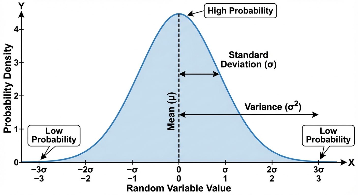
• Gaussian (Normal) Distribution: The most common distribution in ML. It is defined by the Bell Curve.
  • Notation:
  • Defined by Mean () and Variance ().

2.3 Statistical Measures

• Mean ( or ): The expected value or average of the random variable. It represents the central tendency.
• Variance ( or ): Measures the spread or dispersion of the data points around the mean.
  
• Covariance: Measures the joint variability of two random variables ( and ).
  • Positive Covariance: Variables move in the same direction.
  • Negative Covariance: Variables move in opposite directions.
  • Zero Covariance: Variables are linearly independent.

2.4 Types of Probability

• Marginal Probability (): The probability of an event irrespective of the outcome of other variables (Sum rule).
• Joint Probability (): The probability of two (or more) events happening at the same time ( AND ).
• Conditional Probability (): The probability of an event occurring given that event has already occurred.
  

3. Bayes’ Theorem and Inference

Bayes' Theorem describes the probability of an event, based on prior knowledge of conditions that might be related to the event. It is the foundation of Bayesian Inference and Naive Bayes classifiers.

3.1 The Theorem

Where:

• (Posterior): Probability of hypothesis being true given observed evidence .
• (Likelihood): Probability of observing evidence given that hypothesis is true.
• (Prior): Probability of hypothesis being true before observing evidence.
• (Evidence): Total probability of observing the evidence.

3.2 Likelihood vs. Probability

Though used interchangeably in common language, they are distinct in statistics:

• Probability: Used when the parameters of the distribution are known, and we want to predict the outcome of future data.
• Likelihood: Used when the data is observed, and we want to estimate the parameters that most likely produced this data. This leads to Maximum Likelihood Estimation (MLE).

4. Calculus for Machine Learning

Calculus is primarily used in ML for optimization. We use it to minimize the "loss" or "error" of a model by adjusting its weights.

4.1 Functions

A function maps input variables to an output. In ML, the most important function is the Loss Function (or Cost Function), denoted as . It maps the model parameters () to a scalar value representing error.

4.2 Partial Derivatives

When a function depends on multiple variables (e.g., multiple weights in a neural network), we calculate the derivative with respect to one variable while treating the others as constants.

• Notation: (read as "partial of f with respect to x").

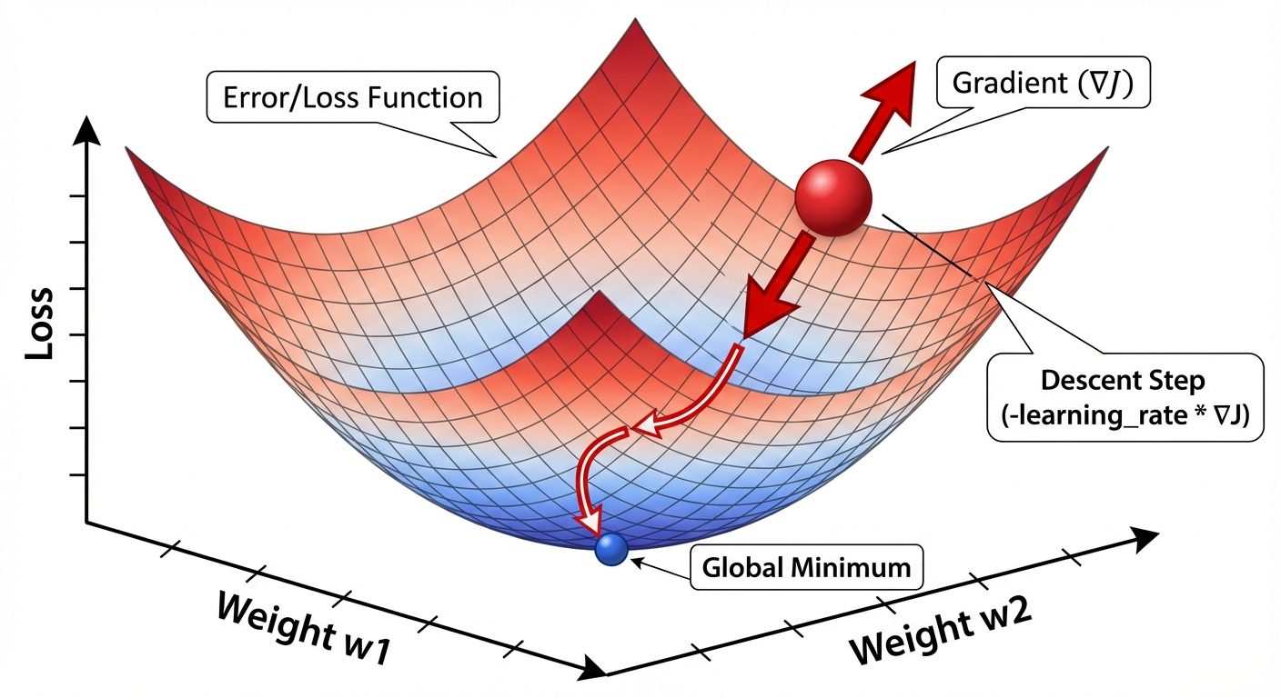
4.3 The Gradient

The gradient is a vector containing all the partial derivatives of a function.

• Symbol: (nabla).
• For a function , the gradient is:
  
• Key Property: The gradient vector points in the direction of the steepest ascent (greatest increase) of the function.
• Gradient Descent: To minimize loss, we move in the direction opposite to the gradient:
  
  
  (Where is the learning rate).

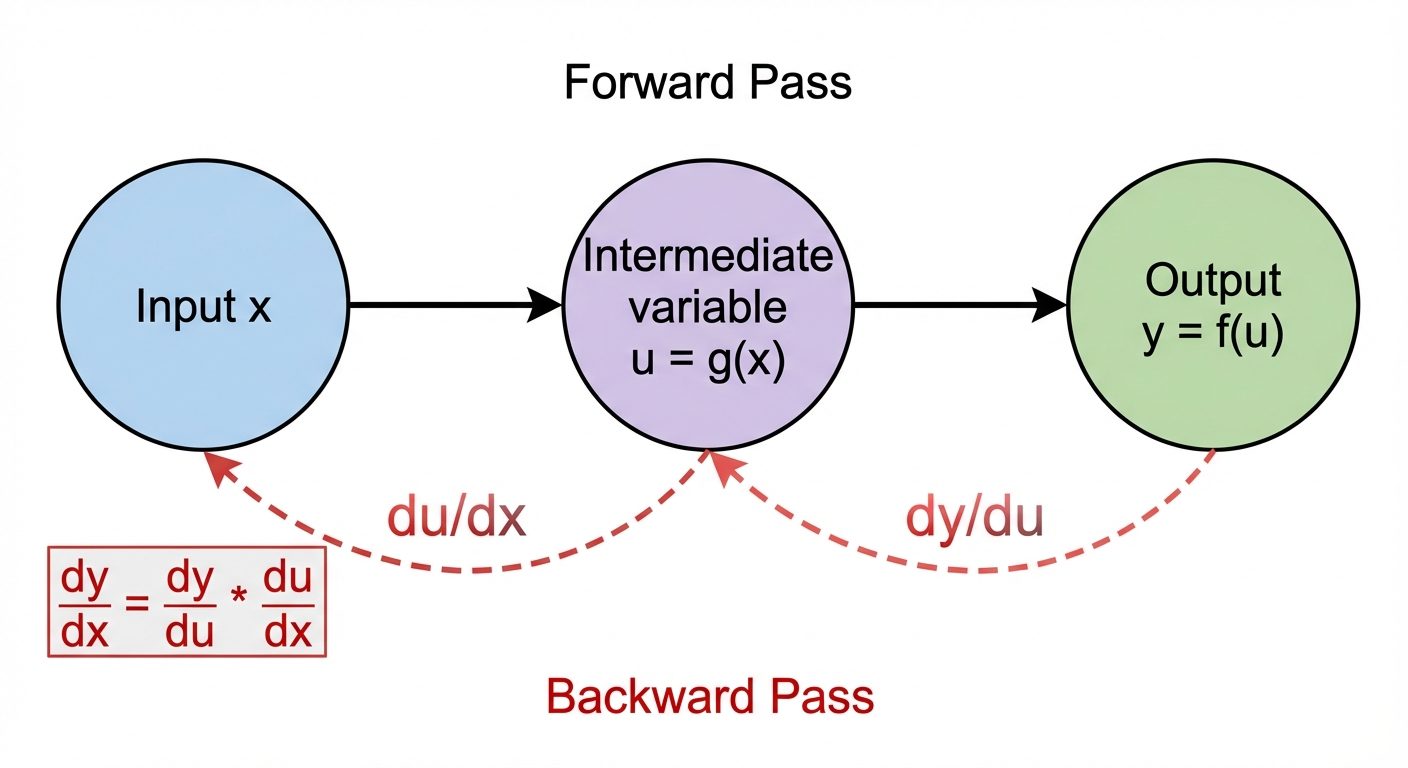
4.4 The Chain Rule

The Chain Rule is the formula for computing the derivative of the composition of two or more functions.

• Formula: If and , then:
  
• Importance in ML: This is the mathematical engine behind Backpropagation. Neural networks are essentially nested composite functions (). To update weights in the first layer, we must calculate how they affect the output by multiplying derivatives "chain-linked" from the output back to the input.