Unit 6 - Notes
Unit 6: Statistical Learning Theory
1. Well-Posed Learning Problems
A computer program is said to learn from experience with respect to some class of tasks and performance measure , if its performance at tasks in , as measured by , improves with experience .
Components of the Definition (The T-P-E Framework)
- Task (): The specific behavior or function the system must perform (e.g., recognizing faces, playing chess, filtering spam).
- Performance Measure (): A quantitative metric used to evaluate how well the system performs the task (e.g., accuracy, mean squared error, win rate).
- Experience (): The data or interactions the system uses to learn (e.g., labeled image datasets, history of past games).
Example: Spam Filtering
- Task (): Classify emails as "Spam" or "Not Spam."
- Performance (): Percentage of emails correctly classified.
- Experience (): A database of emails labeled by humans.
2. Components of a Learning System
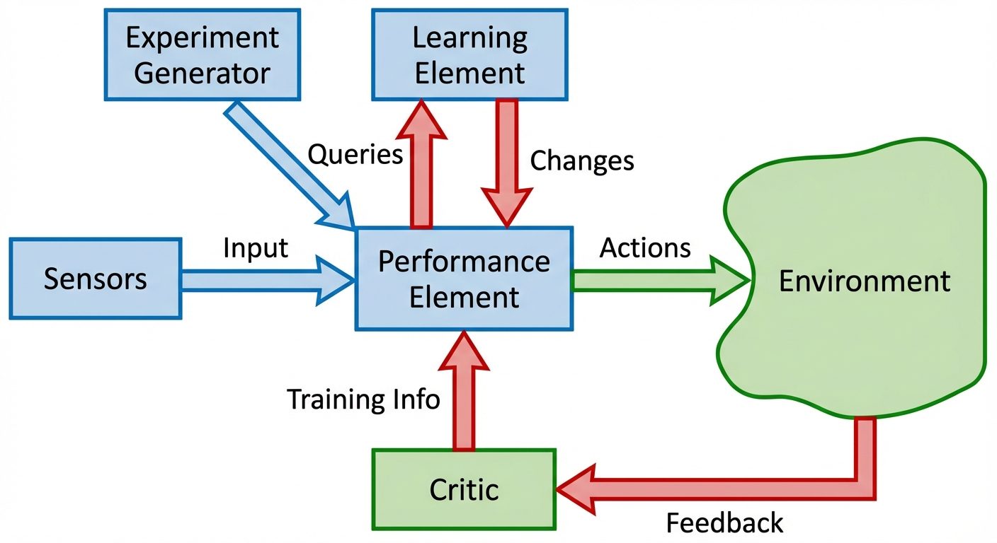
Designing a learning system requires distinct functional modules that interact to convert raw data into a refined hypothesis.
Key Functional Components
- The Critic (Evaluator): Compares the output of the learner against the ground truth or a performance standard. It produces an error signal or reward.
- The Learner (Performance Element): The core algorithm that estimates the target function. It takes feedback from the critic to adjust internal parameters.
- The Generalizer (Hypothesis Generator): Takes specific training examples and outputs a hypothesis that covers unseen cases.
- The Experiment Generator: (In active learning) Decides what new example the system should investigate next to maximize learning.
3. Statistical Learning Framework
Statistical Learning Theory (SLT) provides the mathematical foundation for analyzing machine learning algorithms. It formalizes the problem of inference from data.
Formal Definitions
- Input Space (): The set of all possible inputs (feature vectors).
- Output Space (): The set of all possible outputs (labels).
- Unknown Distribution (): A fixed but unknown probability distribution over . We assume data is generated i.i.d (independent and identically distributed) from .
- Target Function (): The ideal function that we want to approximate.
- Hypothesis Space (): The set of all functions the algorithm can select from (e.g., the set of all linear classifiers).
- Loss Function (): A function that measures the penalty for predicting when the true label is .
The Goal
The goal is to find a hypothesis that minimizes the Risk (Expected Error) over the unknown distribution:
4. Empirical Risk Minimization (ERM)
Since we do not know the distribution , we cannot calculate the true risk . Instead, we rely on the training data.
Empirical Risk
Given a training set , the empirical risk is the average error on this specific sample:
The ERM Principle
The principle of ERM states that the learning algorithm should choose the hypothesis that minimizes the empirical risk:
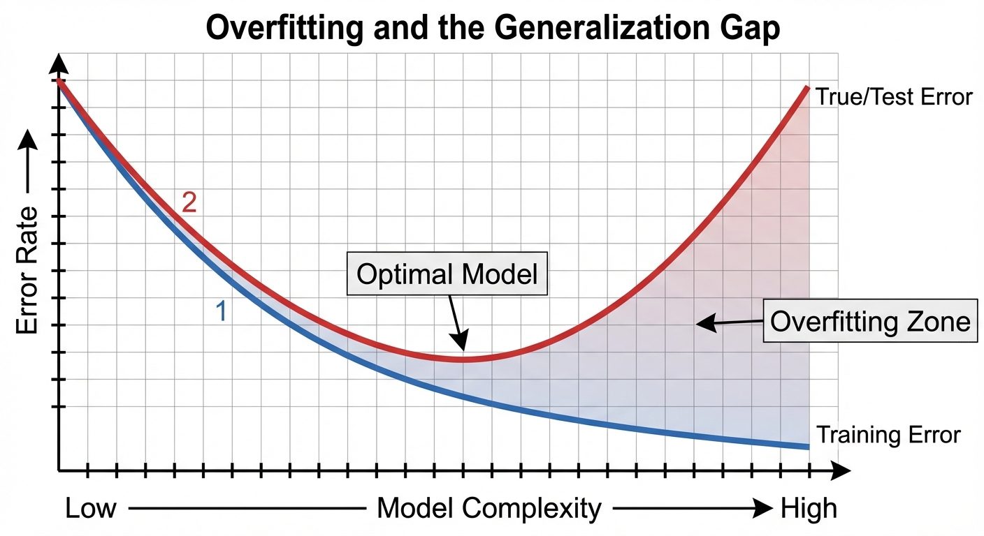
Overfitting and Generalization
Minimizing empirical risk blindly can lead to overfitting. A model might memorize the noise in the training set () but fail on new data ( is high). This difference is the Generalization Gap.
To prevent this, we often use Structural Risk Minimization (SRM), which adds a regularization term to penalize complexity.
5. Inductive Bias
Inductive bias refers to the set of assumptions that the learner uses to predict outputs for inputs that it has not encountered.
Why is it Necessary?
Without inductive bias, a learner cannot generalize. If a learner makes no assumptions, it can only categorize data it has already seen (rote learning). This is often summarized as: "Bias is required for generalization."
Types of Inductive Bias
- Restriction Bias (Language Bias):
- Limits the set of hypotheses considered ().
- Example: Assuming the decision boundary is linear (ignoring all non-linear possibilities).
- Preference Bias (Search Bias):
- Determines how the algorithm searches through . It prefers certain hypotheses over others within the same space.
- Example: Occam's Razor (preferring simpler trees in Decision Tree learning) or Gradient Descent (preferring the nearest local minimum).
6. Role of Prior Knowledge
Prior knowledge complements data. In statistical learning, prior knowledge is injected into the system via:
- Choice of Hypothesis Space: We choose Neural Networks for images because we believe spatial hierarchy matters.
- Regularization: We impose constraints (e.g., L2 regularization) because we assume smoother functions are more likely to be true.
- Bayesian Priors: Explicitly assigning probabilities to hypotheses before seeing data ().
7. Probably Approximately Correct (PAC) Learning
PAC Learning is a framework proposed by Leslie Valiant to mathematically analyze the feasibility of learning. It answers: Under what conditions is learning possible?
The Definition
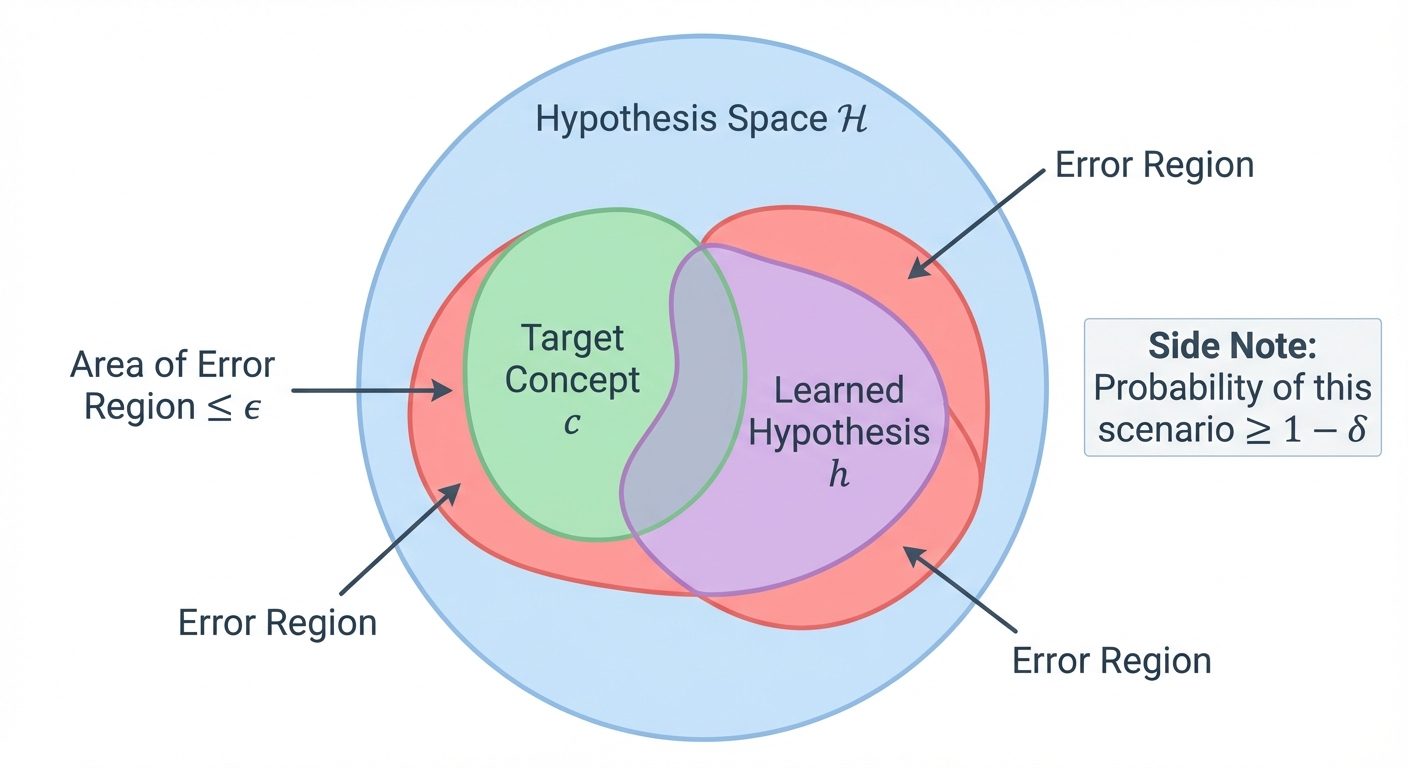
A concept class is PAC-learnable if there exists an algorithm such that:
For any (error parameter) and (confidence parameter), and for any distribution , the algorithm produces a hypothesis such that:
using a sample size polynomial in and .
Interpretation
- Probably (): The algorithm is usually successful (high confidence).
- Approximately (): The error is small (high accuracy).
- We cannot guarantee 0 error or 100% success because the training sample might be unrepresentative (e.g., drawing 100 "heads" in a row from a fair coin).
8. Sample Complexity
Sample complexity refers to the number of training examples required to learn a target function to a desired level of accuracy () and confidence ().
Finite Hypothesis Space
For a finite hypothesis space , the sample complexity to guarantee a consistent learner is PAC is:
- This shows that the number of samples grows linearly with the log of the hypothesis space size.
Infinite Hypothesis Space (VC Dimension)
If is infinite (e.g., neural networks), we use the Vapnik-Chervonenkis (VC) Dimension. The VC dimension measures the capacity (complexity) of the hypothesis space.
- Higher complexity models (high VC dim) require more data to generalize.
9. No Free Lunch Theorem (NFL)
The No Free Lunch theorem (Wolpert, 1996) states that: Averaged over all possible data generating distributions, every classification algorithm has the same error rate when classifying previously unobserved points.
Implications
- No Universal Best Algorithm: There is no single algorithm (e.g., Random Forest, Deep Learning) that works best on every problem.
- Assumptions Matter: An algorithm performs well on a specific task only because its inductive bias matches the properties of that specific task.
- Random Guessing: Averaged over all possible problems (including completely random noise), a sophisticated algorithm performs no better than random guessing. We succeed in the real world because real-world problems are not random; they have structure.
10. Choosing Algorithms Based on Data and Assumptions
Because of the NFL theorem, algorithm selection must be based on the characteristics of the data and domain knowledge.
| Factor | Guideline for Algorithm Selection |
|---|---|
| High Bias vs. High Variance | Use simpler models (Linear Regression, Naive Bayes) for small data to avoid variance. Use complex models (Deep Learning, Boosted Trees) for massive data to reduce bias. |
| Interpretability | If logic must be explained (e.g., medical, legal), use Decision Trees or Linear Models over Black-box Neural Networks. |
| Dimensionality | High dimensional sparse data (text) often works well with Linear SVMs. Low dimensional dense data works well with KNN or Neural Nets. |
| Prior Knowledge | If valid assumptions exist (e.g., image data has spatial locality), use algorithms with matching bias (e.g., Convolutional Neural Networks). |
The Occam's Razor Principle
When choosing between two hypotheses that explain the data equally well, choose the simpler one. Simpler models are less likely to overfit (lower VC dimension) and require less sample complexity.