Back to Subject

Practice MCQ Subjective

Unit 1 - Notes

PHY110 8 min read

Unit 1: Electromagnetic theory

1. Fundamentals of Vector Calculus

To understand electromagnetic theory, one must first master the mathematical tools used to describe fields.

1.1 Scalar and Vector Fields

Scalar Field: A region of space where a scalar quantity relates to every point. The magnitude depends on position coordinates .
- Examples: Temperature distribution in a room, Electric Potential ( $V$ ), Density.
- Notation: $\phi(x, y, z)$ .
Vector Field: A region where a vector quantity (magnitude and direction) relates to every point.
- Examples: Velocity of fluid flow, Electric Field intensity ( $\vec{E}$ ), Magnetic Field intensity ( $\vec{H}$ ).
- Notation: $\vec{A}(x, y, z) = A_x\hat{i} + A_y\hat{j} + A_z\hat{k}$ .

1.2 The Del Operator ( $\nabla$ )

The vector differential operator used to perform gradient, divergence, and curl operations:

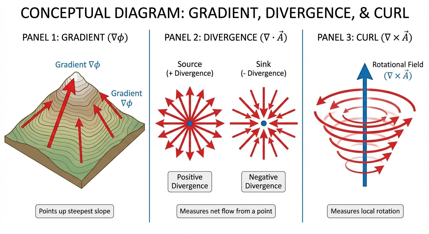
\nabla = \hat{i}\frac{\partial}{\partial x} + \hat{j}\frac{\partial}{\partial y} + \hat{k}\frac{\partial}{\partial z}

1.3 Gradient, Divergence, and Curl

Gradient (Grad $\phi$ )

The gradient operates on a scalar field and results in a vector field. It represents the maximum rate of change (steepest slope) of the scalar function and points in the direction of that change.

\nabla \phi = \hat{i}\frac{\partial \phi}{\partial x} + \hat{j}\frac{\partial \phi}{\partial y} + \hat{k}\frac{\partial \phi}{\partial z}

Physical Significance: In electrostatics, the Electric Field is the negative gradient of Potential: $\vec{E} = -\nabla V$ .

Divergence (Div $\vec{A}$ )

Divergence operates on a vector field and results in a scalar. It measures the net outflow of a vector flux from a small volume.

\nabla \cdot \vec{A} = \frac{\partial A_x}{\partial x} + \frac{\partial A_y}{\partial y} + \frac{\partial A_z}{\partial z}

Physical Significance:
- Positive Divergence: The point is a source (flux lines originate here).
- Negative Divergence: The point is a sink (flux lines terminate here).
- Zero Divergence: The field is Solenoidal (incompressible flow; lines do not start or stop).

Curl (Curl $\vec{A}$ )

Curl operates on a vector field and results in a vector. It measures the rotation or "swirl" of the field.

\nabla \times \vec{A} = \left| \begin{matrix} \hat{i} & \hat{j} & \hat{k} \\ \frac{\partial}{\partial x} & \frac{\partial}{\partial y} & \frac{\partial}{\partial z} \\ A_x & A_y & A_z \end{matrix} \right|

Physical Significance:
- If $\nabla \times \vec{A} \neq 0$ , the field is rotational.
- If $\nabla \times \vec{A} = 0$ , the field is Irrotational (conservative field).

A comprehensive conceptual diagram divided into three panels demonstrating Gradient, Divergence, and... — AI-generated image — may contain inaccuracies

2. Fundamental Theorems (Qualitative)

These theorems relate line, surface, and volume integrals, allowing conversion between differential and integral forms of Maxwell's equations.

2.1 Gauss’s Divergence Theorem

Relates a Volume Integral to a Surface Integral.

Statement: The volume integral of the divergence of a vector field $\vec{A}$ taken over a volume $V$ is equal to the surface integral of the vector field $\vec{A}$ taken over the closed surface $S$ enclosing that volume.
Mathematical Form:
$\iiint_V (\nabla \cdot \vec{A}) \, dV = \oiint_S \vec{A} \cdot d\vec{S}$
Qualitative Meaning: The total amount of "stuff" (flux) being created inside a box (divergence sum) equals the total amount of "stuff" pushing out through the walls of the box (surface flux).

2.2 Stokes’ Theorem

Relates a Surface Integral to a Line Integral.

Statement: The surface integral of the curl of a vector field $\vec{A}$ over an open surface $S$ is equal to the line integral of the vector field $\vec{A}$ along the closed curve $C$ bounding the surface.
Mathematical Form:
$\iint_S (\nabla \times \vec{A}) \cdot d\vec{S} = \oint_C \vec{A} \cdot d\vec{l}$
Qualitative Meaning: Summing the "swirls" (micro-rotations) inside a surface area cancels out everywhere except at the edge, where it equals the circulation along the boundary path.

3. Poisson and Laplace Equations

These equations are derived from Gauss's Law for Electrostatics ( $\nabla \cdot \vec{E} = \frac{\rho}{\epsilon_0}$ ) and the gradient relationship ( $\vec{E} = -\nabla V$ ).

3.1 Poisson’s Equation

Describes the potential distribution in a region containing charge.

Substituting $\vec{E} = -\nabla V$ into Gauss's Law:
$\nabla \cdot (-\nabla V) = \frac{\rho}{\epsilon_0}$
$\nabla^2 V = -\frac{\rho}{\epsilon_0}$
Where $\nabla^2$ is the Laplacian operator, $\rho$ is charge density, and $\epsilon_0$ is permittivity.

3.2 Laplace’s Equation

A special case of Poisson’s equation for a charge-free region ( $\rho = 0$ ).

\nabla^2 V = 0

This equation is fundamental in finding the electric potential in regions between conductors (dielectrics/free space).

4. Continuity Equation

The continuity equation represents the Law of Conservation of Charge.

4.1 Statement and Derivation

The net current flowing out of a closed surface must equal the rate of decrease of the positive charge within the volume.

I = \oint_S \vec{J} \cdot d\vec{S} = -\frac{dQ}{dt}

Using Divergence Theorem and

Q = \int_V \rho \, dV

\int_V (\nabla \cdot \vec{J}) \, dV = -\frac{\partial}{\partial t} \int_V \rho \, dV

\nabla \cdot \vec{J} + \frac{\partial \rho}{\partial t} = 0

$\vec{J}$ : Current density
$\rho$ : Volume charge density
Significance: Charge cannot be created or destroyed; if charge moves away from a point (divergence of current), the charge density at that point must decrease.

5. Ampere’s Law and Maxwell’s Modification

5.1 Ampere’s Circuital Law (Static Case)

It states that the line integral of magnetic field intensity $\vec{H}$ around a closed path is equal to the current enclosed by the path.

\nabla \times \vec{H} = \vec{J} \quad \text{(Differential form)}

\oint \vec{H} \cdot d\vec{l} = I_{enclosed} \quad \text{(Integral form)}

5.2 The Inconsistency

If we apply divergence to Ampere's law:

\nabla \cdot (\nabla \times \vec{H}) = \nabla \cdot \vec{J}

Since the divergence of a curl is always zero, this implies

\nabla \cdot \vec{J} = 0

.
However, the continuity equation states

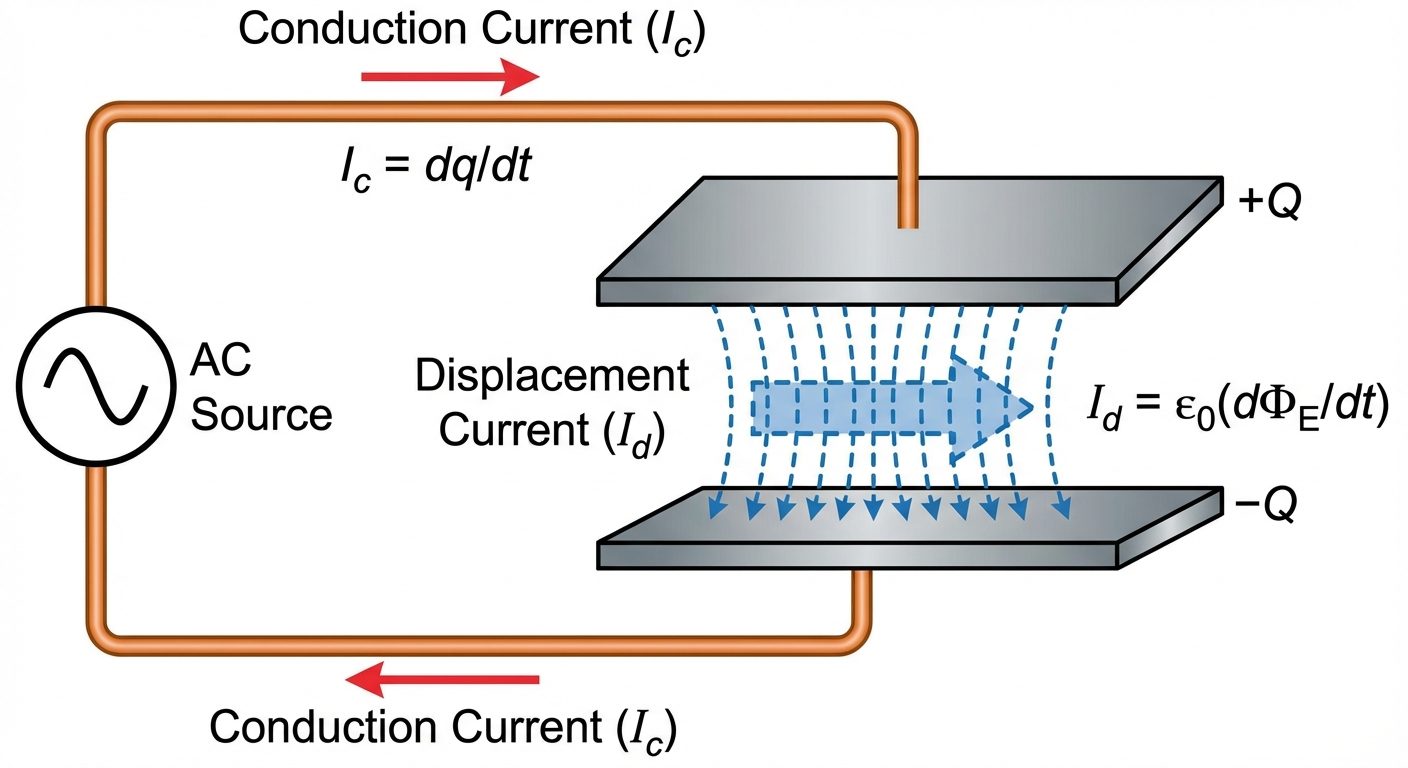
\nabla \cdot \vec{J} = -\frac{\partial \rho}{\partial t}

Contradiction: Ampere's law assumes currents are steady (static). It fails for time-varying fields (like charging a capacitor) where $\frac{\partial \rho}{\partial t} \neq 0$ .

5.3 Maxwell’s Displacement Current

Maxwell suggested adding a term $\vec{J_d}$ (Displacement Current Density) to fix the equation:

\nabla \times \vec{H} = \vec{J_c} + \vec{J_d}

To satisfy continuity,

\vec{J_d}

was identified as the time-varying electric flux density:

\vec{J_d} = \frac{\partial \vec{D}}{\partial t}

Total Current = Conduction Current ( $I_c$ ) + Displacement Current ( $I_d$ )

A detailed circuit diagram showing a parallel plate capacitor connected to an AC voltage source. The... — AI-generated image — may contain inaccuracies

5.4 Modified Ampere’s Law

\nabla \times \vec{H} = \vec{J} + \frac{\partial \vec{D}}{\partial t}

This equation implies that a changing electric field produces a magnetic field, just as a conduction current does.

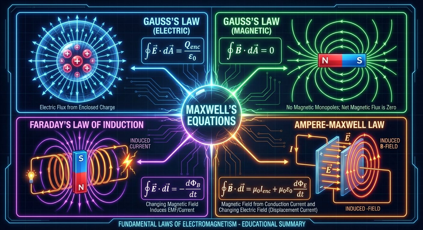
6. Maxwell’s Electromagnetic Equations

Maxwell unified electricity and magnetism into four equations that describe all electromagnetic phenomena.

6.1 The Equations (Table)

No.	Name	Differential Form	Integral Form	Physical Significance
1	Gauss’s Law for Electrostatics	$\nabla \cdot \vec{D} = \rho$	$\oiint \vec{D} \cdot d\vec{S} = Q_{enc}$	Electric flux diverging from a volume equals the charge enclosed. Sources of E-field are charges.
2	Gauss’s Law for Magnetism	$\nabla \cdot \vec{B} = 0$	$\oiint \vec{B} \cdot d\vec{S} = 0$	Magnetic monopoles do not exist. Magnetic field lines are continuous loops (Solenoidal).
3	Faraday’s Law of Induction	$\nabla \times \vec{E} = -\frac{\partial \vec{B}}{\partial t}$	$\oint \vec{E} \cdot d\vec{l} = -\frac{d\Phi_B}{dt}$	A time-varying magnetic field produces a circulating electric field (EMF).
4	Modified Ampere’s Law	$\nabla \times \vec{H} = \vec{J} + \frac{\partial \vec{D}}{\partial t}$	$\oint \vec{H} \cdot d\vec{l} = I + \int \frac{\partial \vec{D}}{\partial t} \cdot d\vec{S}$	Magnetic fields are produced by both conduction currents AND time-varying electric fields.

Constitutive Relations:

$\vec{D} = \epsilon \vec{E}$ (Electric Flux Density)
$\vec{B} = \mu \vec{H}$ (Magnetic Flux Density)
$\vec{J} = \sigma \vec{E}$ (Ohm's Law at a point)

A conceptual 4-quadrant infographic summarizing Maxwell's Equations. Quadrant 1 (Gauss Electric): A ... — AI-generated image — may contain inaccuracies

6.2 Physical Significance of Maxwell's Equations

Static vs. Dynamic: Equations 1 & 2 are static (divergence) equations. Equations 3 & 4 are dynamic (curl) equations involving time derivatives.
Wave Propagation: Equations 3 and 4 are "coupled." A changing $\vec{B}$ creates an $\vec{E}$ (Faraday), and that changing $\vec{E}$ creates a $\vec{B}$ (Ampere-Maxwell). This cycle allows electromagnetic waves to propagate through a vacuum.
Conservation: They embody the conservation of charge and energy within electromagnetic systems.
Symmetry: Maxwell added the displacement current term, introducing symmetry between electric and magnetic fields (both can generate the other).

Unit 2