Unit 4 - Notes

MTH166 6 min read

Unit 4: Partial Differential Equation

1. Introduction to Partial Differential Equations (PDE)

A Partial Differential Equation is an equation involving an unknown function of two or more independent variables and its partial derivatives with respect to those variables.

1.1 Fundamental Concepts

Let $z = f(x, y)$ be a function of two independent variables $x$ and $y$ .
Common notation for partial derivatives:

$p = \frac{\partial z}{\partial x}$
$q = \frac{\partial z}{\partial y}$
$r = \frac{\partial^2 z}{\partial x^2}$
$s = \frac{\partial^2 z}{\partial x \partial y}$
$t = \frac{\partial^2 z}{\partial y^2}$

Order: The order of the highest derivative occurring in the equation.
Degree: The power of the highest order derivative after the equation is cleared of radicals and fractions.

1.2 Classification of Second Order Linear PDEs

The general form of a linear second-order PDE in two variables is:
$A\frac{\partial^2 u}{\partial x^2} + B\frac{\partial^2 u}{\partial x \partial y} + C\frac{\partial^2 u}{\partial y^2} + D\frac{\partial u}{\partial x} + E\frac{\partial u}{\partial y} + Fu = G$

Where $A, B, C, D, E, F, G$ are functions of $x$ and $y$ or constants. The classification depends on the discriminant $\Delta = B^2 - 4AC$ .

A conceptual diagram illustrating the classification of Second Order PDEs. The diagram should be spl... — AI-generated image — may contain inaccuracies

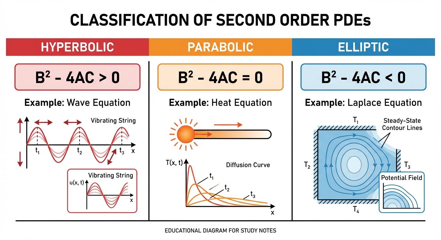
Discriminant	Classification	Prototype Equation	Physical Application
$B^2 - 4AC > 0$	Hyperbolic	Wave Equation	Vibrations, Sound waves
$B^2 - 4AC = 0$	Parabolic	Heat Equation	Diffusion, Heat conduction
$B^2 - 4AC < 0$	Elliptic	Laplace Equation	Steady-state fields, Potential theory

2. Method of Separation of Variables

The method of Separation of Variables is the most common technique for solving linear homogeneous PDEs with specific boundary conditions. It reduces a PDE into a set of Ordinary Differential Equations (ODEs).

2.1 The General Procedure

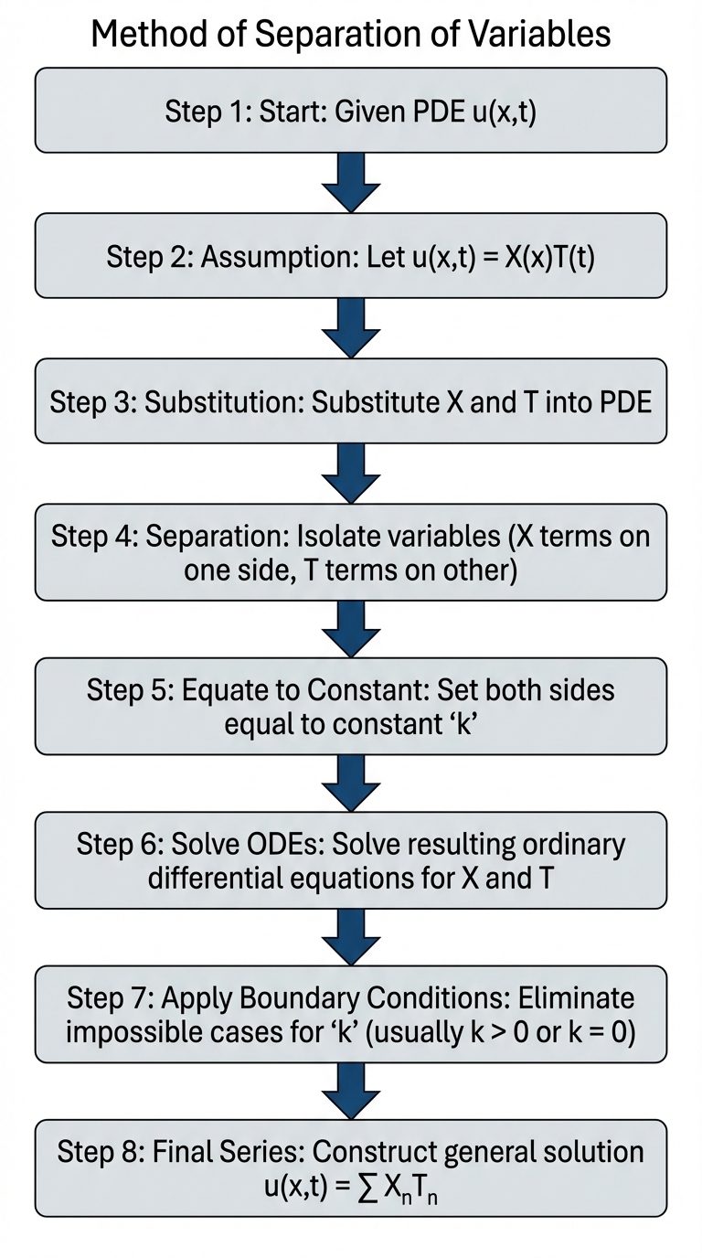
A vertical flowchart diagram detailing the Method of Separation of Variables.
Step 1 Box: "Start: G... — AI-generated image — may contain inaccuracies

2.2 Mathematical Steps

Assume a solution: If dependent variable $u$ depends on $x$ and $t$ , assume $u(x,t) = X(x) \cdot T(t)$ .
Differentiate: Calculate $\frac{\partial u}{\partial x} = X'T$ , $\frac{\partial^2 u}{\partial x^2} = X''T$ , $\frac{\partial u}{\partial t} = XT'$ , etc.
Substitute and Separate: Plug derivatives into the PDE and move all $x$ terms to one side and all $t$ terms to the other.
$\frac{X''}{X} = \frac{T'}{T}$
Introduce Separation Constant: Since and are independent, both sides must equal a constant, say .
- Case 1: $k = p^2$ (Positive) — usually leads to exponential growth (rejected in physical problems requiring stability).
- Case 2: $k = 0$ — leads to linear solutions.
- Case 3: $k = -p^2$ (Negative) — leads to oscillatory (trigonometric) solutions. Most common for Wave/Heat equations.

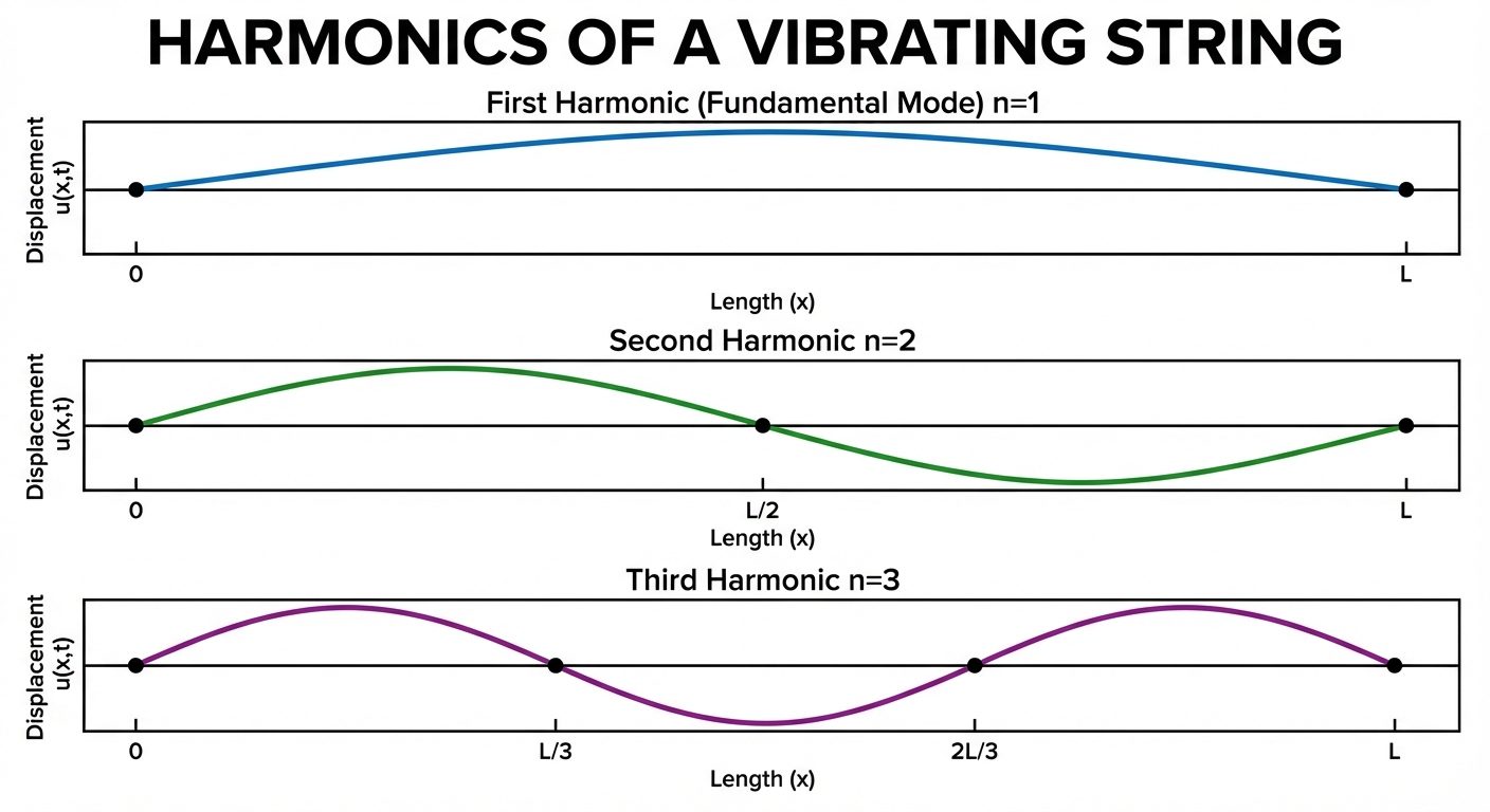
3. Solution of The Wave Equation

The one-dimensional wave equation describes the transverse vibrations of a stretched string.

Equation:
$\frac{\partial^2 u}{\partial t^2} = c^2 \frac{\partial^2 u}{\partial x^2}$
Where $c^2 = \frac{T}{m}$ (Tension / mass per unit length).

3.1 Boundary and Initial Conditions

For a string of length $L$ fixed at both ends:

Boundary Conditions (BCs):
- $u(0, t) = 0$ (Left end fixed)
- $u(L, t) = 0$ (Right end fixed)
Initial Conditions (ICs):
- $u(x, 0) = f(x)$ (Initial shape/displacement)
- $\frac{\partial u}{\partial t}(x, 0) = g(x)$ (Initial velocity)

3.2 Solving Process

Using Separation of Variables with constant $-p^2$ :

ODEs:
- $X'' + p^2 X = 0 \implies X(x) = c_1 \cos(px) + c_2 \sin(px)$
- $T'' + c^2 p^2 T = 0 \implies T(t) = c_3 \cos(cpt) + c_4 \sin(cpt)$
Applying BCs:
- $u(0,t)=0 \implies c_1 = 0$ .
- $u(L,t)=0 \implies c_2 \sin(pL) = 0$ . Since $c_2 \neq 0$ (trivial solution), $\sin(pL) = 0$ .
- Therefore, $pL = n\pi \implies p = \frac{n\pi}{L}$ for $n=1,2,3...$ (Eigenvalues).
General Solution:
$u(x,t) = \sum_{n=1}^{\infty} \left[ A_n \cos\left(\frac{n\pi ct}{L}\right) + B_n \sin\left(\frac{n\pi ct}{L}\right) \right] \sin\left(\frac{n\pi x}{L}\right)$

A detailed diagram showing the "Harmonics of a Vibrating String".
The image should show three verti... — AI-generated image — may contain inaccuracies

4. Solution of The Heat Equation

The one-dimensional heat equation describes the distribution of temperature in a given region over time.

Equation:
$\frac{\partial u}{\partial t} = c^2 \frac{\partial^2 u}{\partial x^2}$
Where $c^2$ is the thermal diffusivity.

4.1 Boundary Conditions

For a rod of length $L$ with ends kept at zero temperature:

BCs: $u(0, t) = 0$ and $u(L, t) = 0$ for all $t$ .
IC: $u(x, 0) = f(x)$ (Initial temperature distribution).

4.2 Solving Process

Separation: leads to and .
- Note: The time equation is First Order.
Solutions:
- $X(x) = c_1 \cos(px) + c_2 \sin(px)$
- $T(t) = c_3 e^{-c^2 p^2 t}$ (Exponential decay).
Applying BCs:
- Similar to the wave equation, $u(0,t)=0$ and $u(L,t)=0$ implies $c_1=0$ and $p = \frac{n\pi}{L}$ .
General Solution:
- Note: As $t \to \infty$ , $u(x,t) \to 0$ (Steady state temperature is 0).

5. Solution of The Laplace Equation

The Laplace equation describes steady-state phenomena (does not depend on time $t$ ). It typically involves two spatial dimensions.

Equation:
$\frac{\partial^2 u}{\partial x^2} + \frac{\partial^2 u}{\partial y^2} = 0$

5.1 Physical Context

Used for solving steady-state heat flow in a rectangular plate or electrostatic potential distributions.

5.2 Solving Process

Using Separation of Variables $u(x,y) = X(x)Y(y)$ :
$\frac{X''}{X} = -\frac{Y''}{Y} = k$

There are three distinct solution types depending on the sign of $k$ . The correct form is chosen based on which direction has zero boundary conditions.

Constant ( $k$ )	Solution for $X(x)$	Solution for $Y(y)$	Usage Heuristic
$k = p^2$	$c_1 e^{px} + c_2 e^{-px}$	$c_3 \cos(py) + c_4 \sin(py)$	Use if BCs on $y$ are 0
$k = -p^2$	$c_1 \cos(px) + c_2 \sin(px)$	$c_3 e^{py} + c_4 e^{-py}$	Use if BCs on $x$ are 0
$k = 0$	$c_1 x + c_2$	$c_3 y + c_4$	Rarely used alone

5.3 Example: Finite Plate

Consider a rectangular plate $0 \le x \le a$ , $0 \le y \le b$ .

BCs: $u(0,y)=0, u(a,y)=0, u(x,0)=0, u(x,b)=f(x)$ .
Since $x=0$ and $x=a$ are zero, we need sinusoidal behavior in $x$ . We choose $k = -p^2$ .
Solution Form:
$u(x,y) = \sum_{n=1}^{\infty} A_n \sin\left(\frac{n\pi x}{a}\right) \sinh\left(\frac{n\pi y}{a}\right)$
(Note: Hyperbolic sine/cosine are preferred for the non-sinusoidal direction in finite plates).

Unit 3

Unit 5