Unit 3 - Notes
Unit 3: Linear Differential Equations
1. Introduction
A linear differential equation of order with constant coefficients is of the form:
Where are constants and is a function of .
General Solution Structure:
The complete solution consists of two parts:
- Complementary Function (C.F.): The solution to the homogeneous equation (where ).
- Particular Integral (P.I.): A specific solution satisfying the non-homogeneous equation.
2. Solution by Operator Method (D-Operator)
We introduce the differential operator . Consequently, , and so on. The differential equation can be written as:
2.1 Finding the Complementary Function (C.F.)
To find the C.F., we solve the Auxiliary Equation (A.E.) obtained by replacing with and equating .
| Nature of Roots () | Form of C.F. |
|---|---|
| Real and Distinct () | |
| Real and Equal () | |
| Complex Conjugates () | |
| Repeated Complex () |
2.2 Finding the Particular Integral (P.I.)
The Particular Integral is given by . The method depends on the form of .
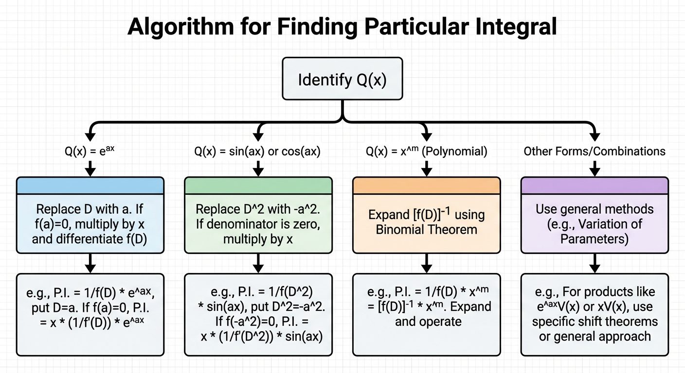
Case I:
- Rule: Replace with .
- Exception: If , then .
Case II: or
- Rule: Replace with .
- Exception: If the denominator becomes zero, multiply by and differentiate the operator with respect to .
Case III: (Algebraic Polynomial)
- Rule: Convert the operator into the form and expand using the Binomial Theorem.
- Expansions:
Case IV:
- Rule (Exponential Shift):
- After shifting to the left, operate on .
Case V:
- Rule:
3. Method of Undetermined Coefficients
This method is used when is a standard function (exponential, polynomial, sinusoidal, or a sum/product of these) and the operator method is either difficult to apply or strictly restricted by the problem statement.
Procedure:
- Find the Complementary Function ().
- Assume a trial solution based on the form of .
- Differentiate and substitute it into the original DE.
- Equate coefficients of like terms to solve for the unknown constants.
Choice of Trial Solution:
| Term in | Assumed Trial Solution |
|---|---|
| () | |
| or |
Modification Rule: If any term in the assumed trial solution is already present in the C.F., multiply the trial solution by (or if the root is repeated).
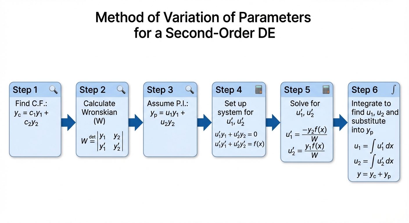
4. Method of Variation of Parameters
This is a general method used to find the particular integral for linear DEs of the form , especially when is not a standard form (e.g., ).
Step 3 Block: "Compute Parameters u and v". Show formulas: u = -Integral[(y_2 R(x)) / W] dx and v = Integral[(y_1 R(x)) / W] dx.
Step 4 Block: "Final Solution". Formula: y_p = u(x)y_1 + v(x)y_2.
Connect blocks with downward arrows. Use a clean, academic layout with math symbols clearly rendered.]
Algorithm:
- Find the C.F.: .
- Calculate the Wronskian ():
- The Particular Integral is given by:
Where:
- General Solution: .
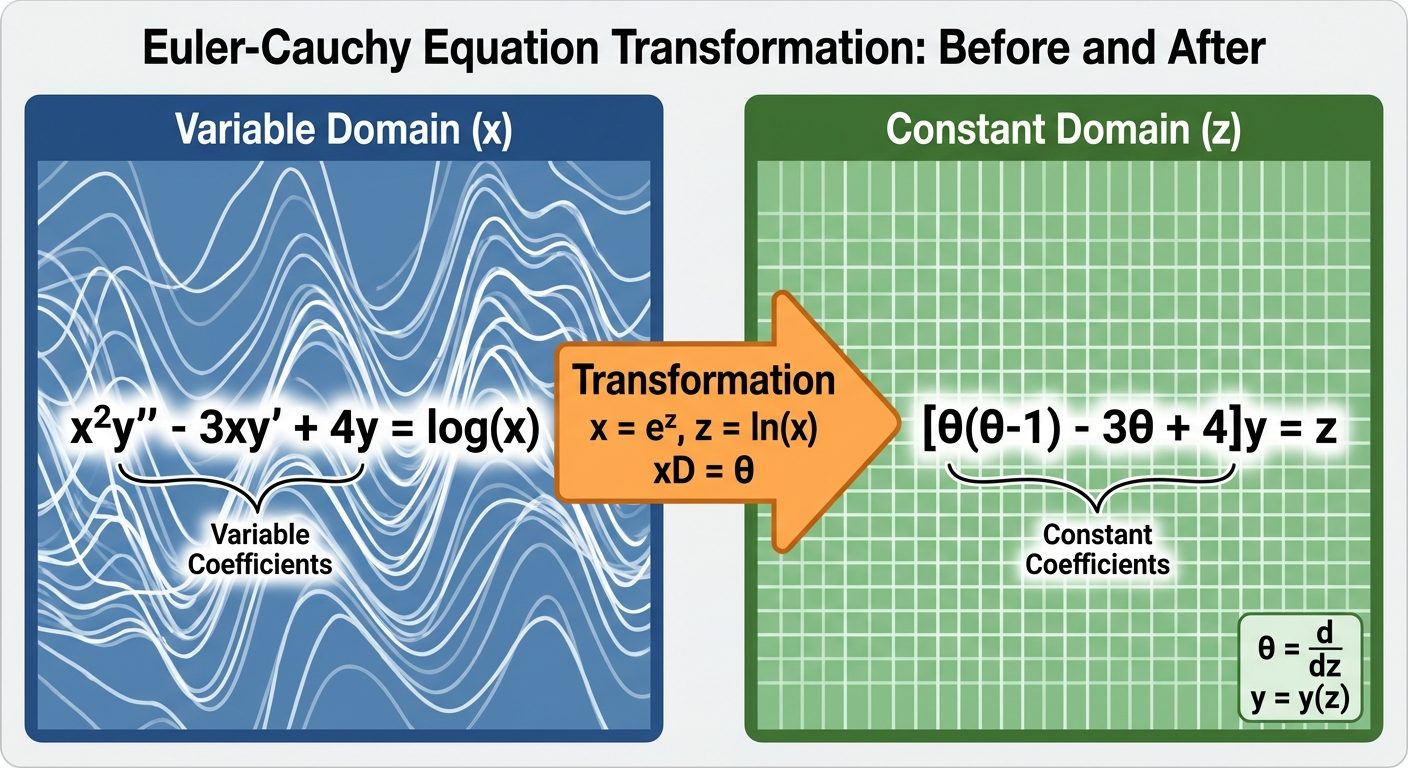
5. Euler-Cauchy Equation (Linear Equation with Variable Coefficients)
Also known as the Homogeneous Linear Equation. It has the form:
Note that the power of matches the order of the derivative.
Transformation Procedure:
To solve, we transform it into a linear DE with constant coefficients.
- Substitution: Let or .
- Operator Transformation:
Define .
Bottom Caption: "Converting Variable Coefficients to Constant Coefficients".]
Steps to Solve:
- Substitute the operators into the equation.
- Replace with the function in terms of (replace with ).
- Solve the resulting constant coefficient DE for .
- Back-substitute to get the final solution .
6. Simultaneous Differential Equations
This involves solving a system of linear differential equations with constant coefficients involving two or more dependent variables (e.g., ) and one independent variable ().
Method of Operators (Elimination Method):
Consider the system:
Steps:
- Write the equations in operator form ().
- Treat the operators and like algebraic coefficients.
- Eliminate one variable (say ) by multiplying equation (1) by and equation (2) by , then subtracting.
- This yields a single DE in terms of and :
- Solve this DE to find .
- Substitute back into one of the original equations (or eliminate similarly) to find .
- Note: Solving separately introduces extra constants. Substitute into the equations to relate the constants of to .
7. Summary of Key Formulae
- Auxiliary Equation: .
- P.I. for : ().
- P.I. for : Replace .
- Wronskian: .
- Variation of Parameters: .
- Euler Substitution: .