Unit 2 - Notes

MTH166 6 min read

Unit 2: Differential equations of higher order

1. Introduction to Linear Differential Equations

A Linear Differential Equation (LDE) is a differential equation in which the dependent variable ( $y$ ) and its derivatives appear only in the first degree and are not multiplied together.

General Form of Linear Differential Equation of Order $n$

The general form of an $n$ -th order linear differential equation is:

$a_n(x) \frac{d^n y}{dx^n} + a_{n-1}(x) \frac{d^{n-1} y}{dx^{n-1}} + \dots + a_1(x) \frac{dy}{dx} + a_0(x) y = Q(x)$

Where:

$a_0, a_1, \dots, a_n$ are constants or functions of $x$ only.
$a_n(x) \neq 0$ .
$Q(x)$ is a function of $x$ (or a constant).

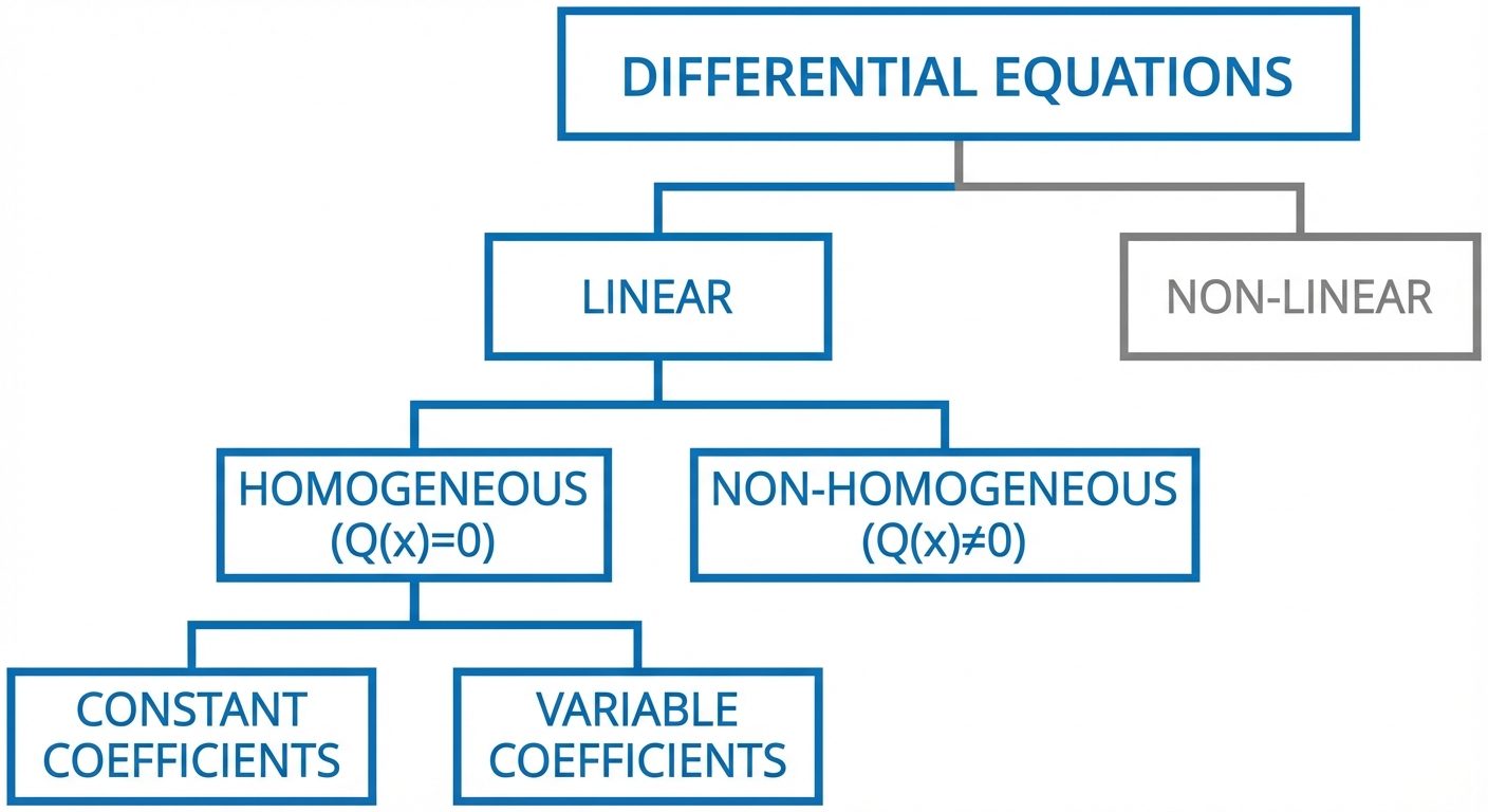
Classification

Homogeneous Linear Differential Equation: If $Q(x) = 0$ .
Non-Homogeneous Linear Differential Equation: If $Q(x) \neq 0$ .
Constant Coefficients: If $a_0, a_1, \dots, a_n$ are real constants.
Variable Coefficients: If any of $a_i$ are functions of $x$ .

A hierarchical tree diagram classifying Differential Equations. The top node is "Differential Equati... — AI-generated image — may contain inaccuracies

2. Linear Dependence and Linear Independence of Solutions

When solving higher-order differential equations, the general solution is constructed from a set of "basis" solutions. It is crucial to determine if these solutions are distinct enough to form a general solution.

Definitions

Let $y_1, y_2, \dots, y_n$ be functions defined on an interval $I$ .

Linearly Dependent (LD): The functions are linearly dependent if there exist constants $c_1, c_2, \dots, c_n$ , not all zero, such that:
$c_1 y_1(x) + c_2 y_2(x) + \dots + c_n y_n(x) = 0$
for all $x$ in $I$ . (Essentially, one function can be written as a combination of others).
Linearly Independent (LI): The functions are linearly independent if the equation:
$c_1 y_1(x) + c_2 y_2(x) + \dots + c_n y_n(x) = 0$
implies that every constant is zero ( $c_1 = c_2 = \dots = c_n = 0$ ).

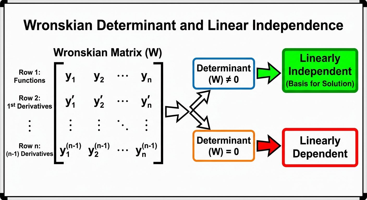
The Wronskian ( $W$ )

The Wronskian determinant is a tool used to test linear independence. For $n$ functions $y_1, y_2, \dots, y_n$ :

$W(y_1, y_2, \dots, y_n) = \begin{vmatrix} y_1 & y_2 & \dots & y_n \\ y_1' & y_2' & \dots & y_n' \\ \vdots & \vdots & \ddots & \vdots \\ y_1^{(n-1)} & y_2^{(n-1)} & \dots & y_n^{(n-1)} \end{vmatrix}$

Theorem:

If $W(x) \neq 0$ for at least one point in the interval, the functions are Linearly Independent.
If the functions are solutions to a homogeneous LDE and $W(x) = 0$ over the interval, the functions are Linearly Dependent.

A visual diagram explaining the Wronskian determinant structure and its outcome. On the left, show t... — AI-generated image — may contain inaccuracies

3. Method of Solution: The Differential Operator ( $D$ )

To simplify the process of solving linear differential equations with constant coefficients, we introduce the Differential Operator notation.

Definition of Operator $D$

Let $D$ denote the operation of differentiation with respect to $x$ :
$D = \frac{d}{dx}, \quad D^2 = \frac{d^2}{dx^2}, \quad \dots, \quad D^n = \frac{d^n}{dx^n}$

Similarly, $\frac{1}{D}$ represents integration:
$\frac{1}{D} f(x) = \int f(x) dx$

Rewriting the Equation

The differential equation:
$a_n \frac{d^n y}{dx^n} + a_{n-1} \frac{d^{n-1} y}{dx^{n-1}} + \dots + a_1 \frac{dy}{dx} + a_0 y = Q(x)$

Can be written as:
$(a_n D^n + a_{n-1} D^{n-1} + \dots + a_1 D + a_0) y = Q(x)$

Or simply:
$f(D)y = Q(x)$

Where $f(D)$ is a polynomial in $D$ .

4. Solution of Homogeneous Linear Differential Equations with Constant Coefficients

A homogeneous linear differential equation with constant coefficients has the form:
$a_n \frac{d^n y}{dx^n} + \dots + a_1 \frac{dy}{dx} + a_0 y = 0$
In operator form: $f(D)y = 0$ .

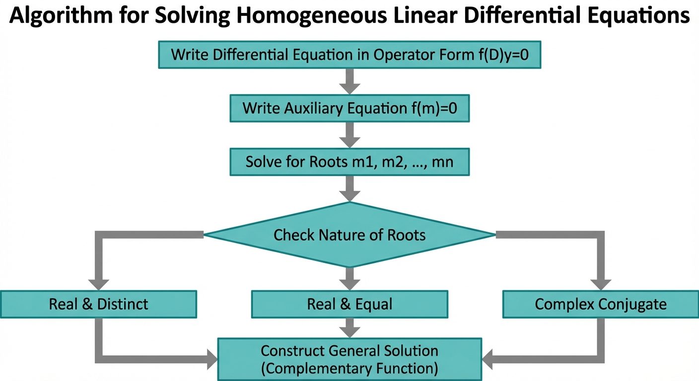
The General Procedure

To solve $f(D)y = 0$ , we rely on the property that exponential functions ( $y = e^{mx}$ ) reproduce themselves upon differentiation.

Assume a trial solution: $y = e^{mx}$ .
Substitute into the equation to get the Auxiliary Equation (A.E.).
- Replacing $D$ with $m$ , we get $f(m) = 0$ .
- $a_n m^n + a_{n-1} m^{n-1} + \dots + a_1 m + a_0 = 0$ .
Find the roots of the Auxiliary Equation ( $m_1, m_2, \dots, m_n$ ).
Write the General Solution based on the nature of the roots.

A vertical flowchart illustrating the algorithm for solving Homogeneous Linear Differential Equation... — AI-generated image — may contain inaccuracies

5. Solution of Second Order Homogeneous LDE

Consider the second-order equation:
$a \frac{d^2 y}{dx^2} + b \frac{dy}{dx} + cy = 0$
Auxiliary Equation: $am^2 + bm + c = 0$ .
Let the roots be $m_1$ and $m_2$ .

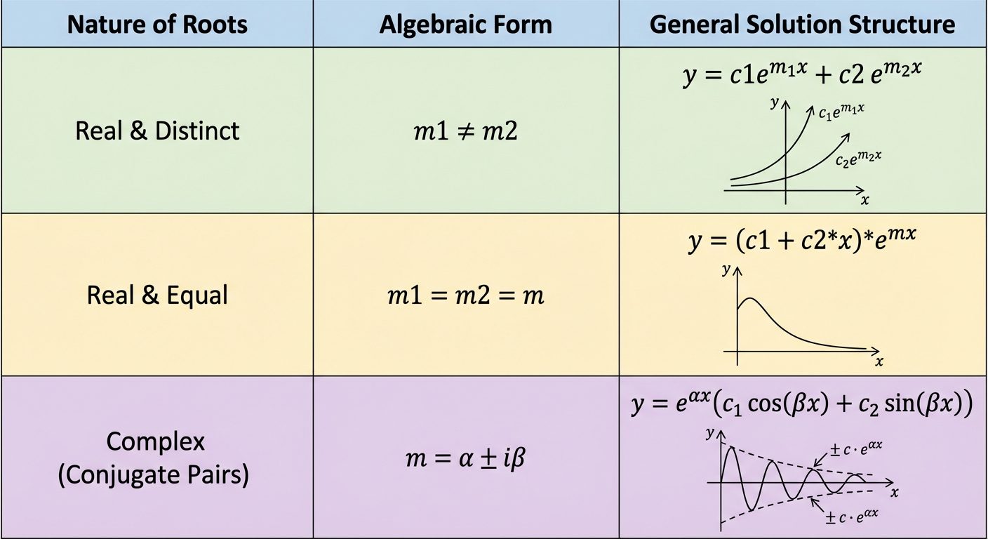
There are three distinct cases for the roots of this quadratic equation:

Case 1: Roots are Real and Distinct ( $m_1 \neq m_2$ )

If the roots are real numbers and not equal, the linearly independent solutions are $e^{m_1 x}$ and $e^{m_2 x}$ .

General Solution:
$y = c_1 e^{m_1 x} + c_2 e^{m_2 x}$

Case 2: Roots are Real and Equal ( $m_1 = m_2 = m$ )

If the discriminant is zero, we have a repeated root $m$ . The first solution is $e^{mx}$ . Through reduction of order, the second independent solution is found to be $x e^{mx}$ .

General Solution:
$y = (c_1 + c_2 x) e^{mx}$

Case 3: Roots are Complex Conjugates ( $m = \alpha \pm i\beta$ )

If the discriminant is negative, roots appear as a pair $\alpha + i\beta$ and $\alpha - i\beta$ .
Using Euler's formula ( $e^{i\theta} = \cos \theta + i \sin \theta$ ), the solution simplifies to trigonometric forms.

General Solution:
$y = e^{\alpha x} (c_1 \cos \beta x + c_2 \sin \beta x)$

$\alpha$ is the real part (governs growth/decay).
$\beta$ is the imaginary part (governs oscillation frequency).

A detailed reference table comparing the three cases of roots for 2nd Order DEs.
Row 1 Header: "Natu... — AI-generated image — may contain inaccuracies

6. Solution of Higher Order Homogeneous LDE with Constant Coefficients

The rules for the second order extend naturally to $n$ -th order equations. We solve the polynomial auxiliary equation of degree $n$ to find $n$ roots.

Rules for Generalization

Distinct Real Roots:
For each distinct real root $m$ , add a term $c e^{mx}$ .
$y = c_1 e^{m_1 x} + c_2 e^{m_2 x} + \dots$
Repeated Real Roots:
If a real root $m$ repeats $k$ times ( $m, m, \dots, m$ ( $k$ times)):
$y = (c_1 + c_2 x + c_3 x^2 + \dots + c_k x^{k-1}) e^{mx}$
Distinct Complex Pair:
For a pair $\alpha \pm i\beta$ :
$y = e^{\alpha x} (c_1 \cos \beta x + c_2 \sin \beta x)$
Repeated Complex Pair:
If the pair $\alpha \pm i\beta$ repeats twice (roots are $\alpha \pm i\beta, \alpha \pm i\beta$ ):
$y = e^{\alpha x} [(c_1 + c_2 x) \cos \beta x + (c_3 + c_4 x) \sin \beta x]$

Example Problem Structure

Problem: Solve $(D^4 - 16)y = 0$ .

Auxiliary Equation: $m^4 - 16 = 0$ .
Factorize: $(m^2 - 4)(m^2 + 4) = 0 \Rightarrow (m-2)(m+2)(m^2+4) = 0$ .
Roots:
- $m = 2$ (Real)
- $m = -2$ (Real)
- $m = \pm 2i$ (Complex conjugate, $\alpha=0, \beta=2$ )
Solution:
Combine the rules:
$y = c_1 e^{2x} + c_2 e^{-2x} + e^{0x}(c_3 \cos 2x + c_4 \sin 2x)$
$y = c_1 e^{2x} + c_2 e^{-2x} + c_3 \cos 2x + c_4 \sin 2x$

Unit 1

Unit 3