Unit 1 - Notes

MTH166 6 min read

Unit 1: Ordinary differential equations

1. Introduction

An Ordinary Differential Equation (ODE) is an equation involving an independent variable ( $x$ ), a dependent variable ( $y$ ), and its derivatives with respect to the independent variable. Unit 1 focuses on first-order differential equations, specifically exact equations, methods to make equations exact, equations of higher degree, and the special case of Clairaut's equation.

2. Exact Differential Equations

Definition

A differential equation of the form:
$M(x, y) dx + N(x, y) dy = 0$
is said to be exact if it can be obtained directly by differentiating a primitive function $u(x, y) = c$ without any subsequent multiplication, elimination, or reduction.

Necessary and Sufficient Condition

The necessary and sufficient condition for the differential equation $M dx + N dy = 0$ to be exact is:
$\frac{\partial M}{\partial y} = \frac{\partial N}{\partial x}$

Where:

$M$ and $N$ are functions of $x$ and $y$ .
$\frac{\partial M}{\partial y}$ is the partial derivative of $M$ with respect to $y$ (treating $x$ as constant).
$\frac{\partial N}{\partial x}$ is the partial derivative of $N$ with respect to $x$ (treating $y$ as constant).

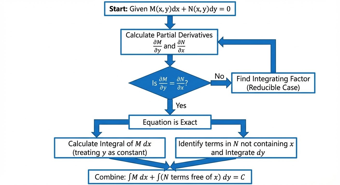
Method of Solution

If the condition of exactness is satisfied, the general solution is given by:

$\int_{y=\text{const}} M dx + \int (\text{terms of } N \text{ free from } x) dy = C$

Step 1: Integrate $M$ with respect to $x$ , treating $y$ as a constant.
Step 2: Integrate only those terms in $N$ that do not contain $x$ , with respect to $y$ .
Step 3: Sum the results and equate to a constant $C$ .

A detailed flowchart diagram illustrating the algorithm for solving Exact Differential Equations. To... — AI-generated image — may contain inaccuracies

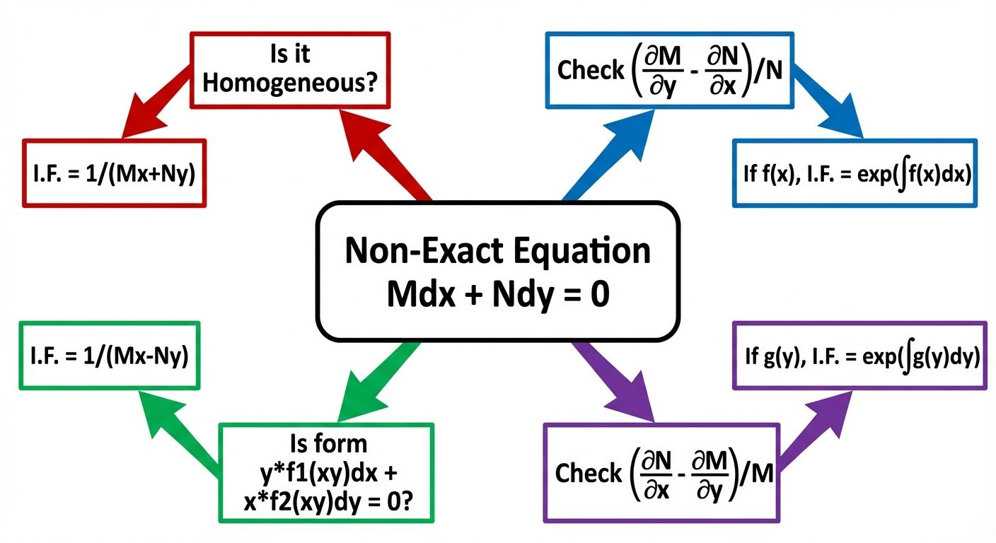
3. Equations Reducible to Exact Equations (Integrating Factors)

If $\frac{\partial M}{\partial y} \neq \frac{\partial N}{\partial x}$ , the equation is not exact. However, it can often be made exact by multiplying it by a function of $x$ and/or $y$ called an Integrating Factor (I.F.).

Rule 1: Homogeneous Equations

If $M dx + N dy = 0$ is a homogeneous equation in $x$ and $y$ (i.e., $M$ and $N$ are homogeneous functions of the same degree), and $Mx + Ny \neq 0$ , then:
$\text{I.F.} = \frac{1}{Mx + Ny}$

Rule 2: Function of product $xy$

If the equation is of the form:
$y \cdot f_1(xy) dx + x \cdot f_2(xy) dy = 0$
and $Mx - Ny \neq 0$ , then:
$\text{I.F.} = \frac{1}{Mx - Ny}$

Rule 3: Function of $x$ alone

If $\frac{\frac{\partial M}{\partial y} - \frac{\partial N}{\partial x}}{N}$ is a function of $x$ only, say $f(x)$ , then:
$\text{I.F.} = e^{\int f(x) dx}$

Rule 4: Function of $y$ alone

If $\frac{\frac{\partial N}{\partial x} - \frac{\partial M}{\partial y}}{M}$ is a function of $y$ only, say $g(y)$ , then:
$\text{I.F.} = e^{\int g(y) dy}$

Rule 5: Equations of the form $x^a y^b (my dx + nx dy) = 0$

For equations reducible to the form $x^h y^k (my dx + nx dy) + x^{h'} y^{k'} (m'y dx + n'x dy) = 0$ , the integrating factor is assumed to be $x^\alpha y^\beta$ . The values of $\alpha$ and $\beta$ are found by applying the condition of exactness to the new equation.

A conceptual decision tree diagram for selecting the correct Integrating Factor. The central node is... — AI-generated image — may contain inaccuracies

4. Equations of the First Order and Higher Degree

These are differential equations where the highest derivative is of the first order ( $\frac{dy}{dx}$ ), but it appears with a power (degree) greater than 1.

Standard Notation: Let $p = \frac{dy}{dx}$ . The general form is:
$p^n + P_1 p^{n-1} + P_2 p^{n-2} + \dots + P_n = 0$
where $P_1, P_2, \dots, P_n$ are functions of $x$ and $y$ .

Case I: Equations Solvable for $p$

If the equation can be resolved into linear factors of $p$ :
$(p - f_1)(p - f_2)\dots(p - f_n) = 0$
Method:

Equate each factor to zero: $p - f_1(x,y) = 0$ , etc.
Solve each first-order ODE individually to get solutions $F_1(x, y, c) = 0$ , $F_2(x, y, c) = 0$ , etc.
The general solution is the product of these solutions:
$F_1(x, y, c) \cdot F_2(x, y, c) \cdot \dots \cdot F_n(x, y, c) = 0$

Case II: Equations Solvable for $y$

The equation can be expressed as $y = F(x, p)$ .
Method:

Differentiate the equation with respect to $x$ .
$\frac{dy}{dx} = p = \phi\left(x, p, \frac{dp}{dx}\right)$
This results in a differential equation in variables $x$ and $p$ .
Solve to find a relation between $x, p, c$ .
Eliminate $p$ between the original equation and the result. If elimination is difficult, express $x$ and $y$ as parametric functions of $p$ .

Case III: Equations Solvable for $x$

The equation can be expressed as $x = F(y, p)$ .
Method:

Differentiate the equation with respect to $y$ .
$\frac{dx}{dy} = \frac{1}{p} = \phi\left(y, p, \frac{dp}{dy}\right)$
This results in a differential equation in variables $y$ and $p$ .
Solve to find a relation between $y, p, c$ .
Eliminate $p$ between the original equation and the result to get the solution in $x$ and $y$ .

5. Clairaut's Equation

Clairaut's equation is a specific type of first-order, higher-degree differential equation.

Standard Form

$y = px + f(p)$
Where $p = \frac{dy}{dx}$ .

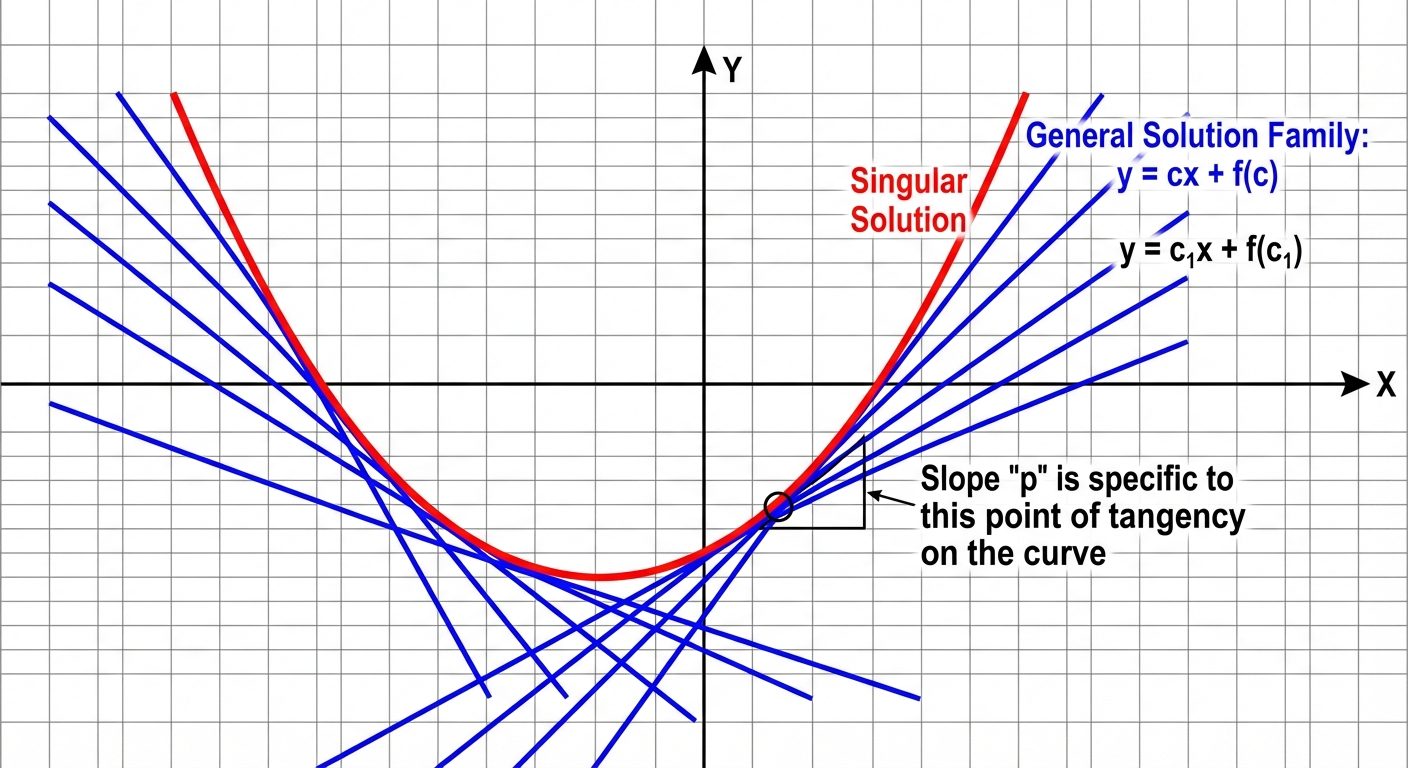
General Solution

The general solution is obtained simply by replacing $p$ with an arbitrary constant $c$ .
Proof Concept:

Differentiate $y = px + f(p)$ with respect to $x$ :
$p = p + x\frac{dp}{dx} + f'(p)\frac{dp}{dx}$
$0 = [x + f'(p)] \frac{dp}{dx}$
Ignoring the factor $[x + f'(p)]$ , we set $\frac{dp}{dx} = 0$ .
Integrating $\frac{dp}{dx} = 0$ gives $p = c$ .
Substituting back:
$y = cx + f(c)$

This represents a family of straight lines.

Singular Solution

The singular solution is a solution that cannot be obtained from the general solution by assigning a value to the constant $c$ . Geometrically, it represents the envelope of the family of straight lines defined by the general solution.

Method to find Singular Solution:

Start with the General Solution: $y = cx + f(c)$ .
Differentiate partially with respect to $c$ :
$0 = x + f'(c)$
Eliminate $c$ between the General Solution equation and the differentiated equation.
The resulting relation between $x$ and $y$ is the singular solution.

An educational geometry diagram explaining Clairaut's Equation. The diagram should show a curve (par... — AI-generated image — may contain inaccuracies

6. Summary of Key Formulas

Type	Form	Solution Method
Exact	$Mdx + Ndy=0$ where $M_y = N_x$	$\int_{y \text{ const}} M dx + \int (\text{terms in } N \text{ w/o } x) dy = C$
Homogeneous	$M, N$ same degree	$I.F. = 1/(Mx+Ny)$
Linear in $y$	$\frac{dy}{dx} + Py = Q$	$y(I.F.) = \int Q(I.F.) dx + C$ , where $I.F. = e^{\int P dx}$
Clairaut's	$y = px + f(p)$	General: $y = cx + f(c)$ ; Singular: Eliminate $c$

Unit 2