Practice MCQ

Unit 1 - Notes

PHY110 8 min read

Unit 1: Electromagnetic Theory

1. Scalar and Vector Fields

Understanding electromagnetic theory requires a foundational knowledge of fields, which describe how physical quantities vary in space and time.

Scalar Field

A region in space where a scalar quantity is defined at every point. It has magnitude but no direction.

Representation: $\phi(x, y, z)$
Examples: Temperature distribution in a metal rod, Electric Potential ( $V$ ), Density of a fluid.
Visual: Represented by level surfaces or contour lines (isotherms, equipotential surfaces).

Vector Field

A region in space where a vector quantity is defined at every point. It possesses both magnitude and direction.

Representation: $\vec{A}(x, y, z) = A_x\hat{i} + A_y\hat{j} + A_z\hat{k}$
Examples: Velocity of fluid flow, Electric Field intensity ( $\vec{E}$ ), Magnetic Field intensity ( $\vec{H}$ ).
Visual: Represented by field lines (flux lines) indicating direction (tangent to line) and magnitude (density of lines).

2. Vector Calculus Operators

The behavior of EM fields is described using the Del operator ( $\nabla$ ), defined as:

\nabla = \frac{\partial}{\partial x}\hat{i} + \frac{\partial}{\partial y}\hat{j} + \frac{\partial}{\partial z}\hat{k}

A. Gradient (Scalar $\to$ Vector)

The gradient of a scalar field $\phi$ represents the maximum rate of change of that scalar function and points in the direction of that maximum increase.

Formula: $\nabla\phi = \frac{\partial \phi}{\partial x}\hat{i} + \frac{\partial \phi}{\partial y}\hat{j} + \frac{\partial \phi}{\partial z}\hat{k}$
Significance in EM: The Electric field is the negative gradient of potential: $\vec{E} = -\nabla V$ .

B. Divergence (Vector $\to$ Scalar)

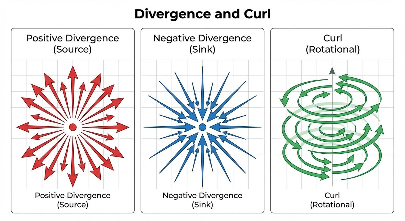
Divergence measures the "outward flux" of a vector field from an infinitesimal volume. It indicates how much a field spreads out (diverges) from a point.

Formula: $\nabla \cdot \vec{A} = \frac{\partial A_x}{\partial x} + \frac{\partial A_y}{\partial y} + \frac{\partial A_z}{\partial z}$
Physical Interpretation:
- Positive Divergence: The point is a Source (lines emerge, e.g., positive charge).
- Negative Divergence: The point is a Sink (lines converge, e.g., negative charge).
- Zero Divergence ( $\nabla \cdot \vec{A} = 0$ ): The field is Solenoidal (incompressible flow, e.g., magnetic fields).

C. Curl (Vector $\to$ Vector)

Curl measures the rotation or "swirling" tendency of a vector field at a point. It represents circulation per unit area.

Formula: $\nabla \times \vec{A} = \begin{vmatrix} \hat{i} & \hat{j} & \hat{k} \\ \frac{\partial}{\partial x} & \frac{\partial}{\partial y} & \frac{\partial}{\partial z} \\ A_x & A_y & A_z \end{vmatrix}$
Physical Interpretation:
- If $\nabla \times \vec{A} \neq 0$ , the field is Rotational (vortex).
- If $\nabla \times \vec{A} = 0$ , the field is Irrotational (conservative, e.g., electrostatic field).

A three-part conceptual diagram illustrating Divergence and Curl side-by-side.
Left panel labeled "... — AI-generated image — may contain inaccuracies

3. Integral Theorems (Qualitative)

These theorems bridge the gap between differential calculus (point-wise) and integral calculus (region-wise).

Gauss’s Divergence Theorem

Relates the flux of a vector field through a closed surface to the divergence of the field inside the enclosed volume.

Statement: The surface integral of the normal component of a vector function $\vec{A}$ over a closed surface $S$ is equal to the volume integral of the divergence of $\vec{A}$ over the volume $V$ enclosed by $S$ .
Mathematical Form:
$\oint_S \vec{A} \cdot d\vec{S} = \int_V (\nabla \cdot \vec{A}) dV$
Utility: Converts Surface Integral $\leftrightarrow$ Volume Integral.

Stokes’ Theorem

Relates the circulation of a vector field along a closed boundary curve to the curl of the field over the open surface bounded by that curve.

Statement: The line integral of a vector function $\vec{A}$ around a closed curve $C$ is equal to the surface integral of the curl of $\vec{A}$ over the open surface $S$ bounded by $C$ .
Mathematical Form:
$\oint_C \vec{A} \cdot d\vec{l} = \int_S (\nabla \times \vec{A}) \cdot d\vec{S}$
Utility: Converts Line Integral $\leftrightarrow$ Surface Integral.

4. Poisson’s and Laplace’s Equations

These are second-order partial differential equations derived from Gauss's Law for electrostatics.

Derivation

From Gauss’s Law: $\nabla \cdot \vec{E} = \frac{\rho}{\epsilon_0}$
From definition of Potential: $\vec{E} = -\nabla V$
Substitute (2) into (1): $\nabla \cdot (-\nabla V) = \frac{\rho}{\epsilon_0} \Rightarrow -\nabla^2 V = \frac{\rho}{\epsilon_0}$

Poisson’s Equation

Used for regions containing charge ( $\rho \neq 0$ ).

\nabla^2 V = -\frac{\rho}{\epsilon_0}

Where $\nabla^2 = \frac{\partial^2}{\partial x^2} + \frac{\partial^2}{\partial y^2} + \frac{\partial^2}{\partial z^2}$ is the Laplacian operator.

Laplace’s Equation

Used for charge-free regions ( $\rho = 0$ ).

\nabla^2 V = 0

This equation implies that the potential in a charge-free region is smooth and has no local maxima or minima.

5. Continuity Equation

The continuity equation represents the Law of Conservation of Charge. It states that the net outward current flow from a closed surface is equal to the rate of decrease of charge within that volume.

Mathematical Derivation

Current $I = \oint_S \vec{J} \cdot d\vec{S}$ (Outward flux of current density).
Rate of decrease of charge: $-\frac{dq}{dt} = -\frac{d}{dt} \int_V \rho dV$ .
Equating them: $\oint_S \vec{J} \cdot d\vec{S} = -\int_V \frac{\partial \rho}{\partial t} dV$ .
Apply Divergence Theorem to LHS: $\int_V (\nabla \cdot \vec{J}) dV = -\int_V \frac{\partial \rho}{\partial t} dV$ .

Final Form

\nabla \cdot \vec{J} + \frac{\partial \rho}{\partial t} = 0

Steady currents ( $\frac{\partial \rho}{\partial t} = 0$ ): $\nabla \cdot \vec{J} = 0$ (Current entering = Current leaving).

6. Ampere’s Circuital Law and Maxwell’s Correction

Ampere's Circuital Law (Original)

The line integral of magnetic field intensity $\vec{H}$ around a closed path is equal to the current enclosed by the path.

Differential Form: $\nabla \times \vec{H} = \vec{J}$

The Inconsistency

Maxwell noticed a mathematical flaw in Ampere's law for time-varying fields.

Take the divergence of Ampere's law: $\nabla \cdot (\nabla \times \vec{H}) = \nabla \cdot \vec{J}$ .
Vector Identity: Divergence of a Curl is always zero. Thus, $\nabla \cdot \vec{J} = 0$ .
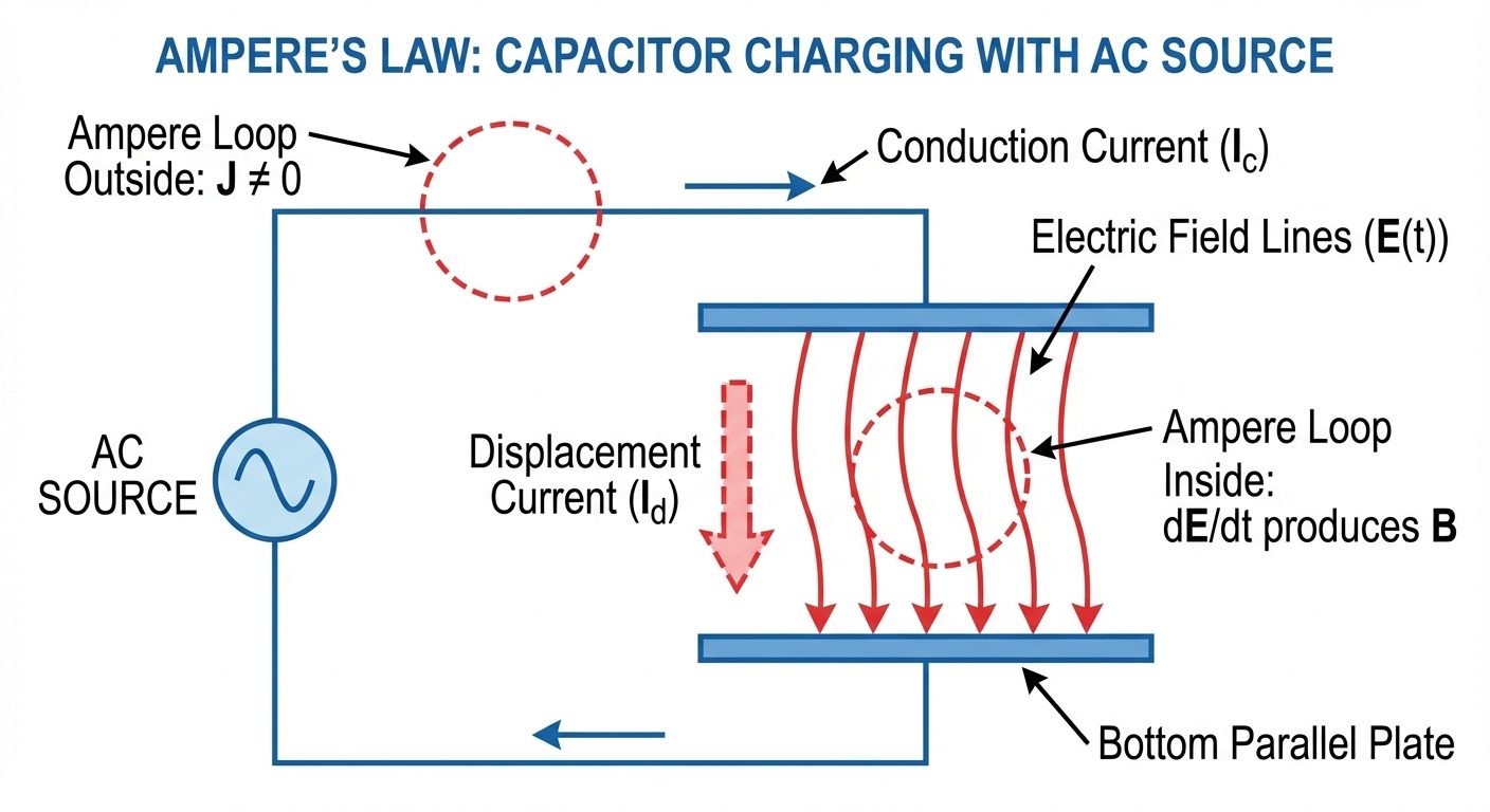
Contradiction: This contradicts the Continuity Equation ( $\nabla \cdot \vec{J} = -\frac{\partial \rho}{\partial t}$ ), which is non-zero for time-varying fields (like charging a capacitor).

Maxwell’s Displacement Current

To fix this, Maxwell added a term $\vec{J_d}$ to the current density.

Modified equation: $\nabla \times \vec{H} = \vec{J} + \vec{J_d}$ .
Using Gauss Law ( $\nabla \cdot \vec{D} = \rho$ ), he derived that $\vec{J_d} = \frac{\partial \vec{D}}{\partial t}$ .

Displacement Current ( $I_d$ ): It is not a flow of physical charge but a time-varying electric field that produces a magnetic field.

I_d = \epsilon_0 \frac{d\phi_E}{dt}

A detailed schematic diagram of a parallel plate capacitor circuit being charged by an AC source.
T... — AI-generated image — may contain inaccuracies

7. Maxwell’s Electromagnetic Equations

Maxwell unified electricity and magnetism into four fundamental equations.

No.	Name	Differential Form	Integral Form
1	Gauss’s Law (Electrostatics)	$\nabla \cdot \vec{D} = \rho$	$\oint_S \vec{D} \cdot d\vec{S} = \int_V \rho dV = Q_{enc}$
2	Gauss’s Law (Magnetism)	$\nabla \cdot \vec{B} = 0$	$\oint_S \vec{B} \cdot d\vec{S} = 0$
3	Faraday’s Law of Induction	$\nabla \times \vec{E} = -\frac{\partial \vec{B}}{\partial t}$	$\oint_C \vec{E} \cdot d\vec{l} = -\frac{d}{dt}\int_S \vec{B} \cdot d\vec{S}$
4	Ampere-Maxwell Law	$\nabla \times \vec{H} = \vec{J} + \frac{\partial \vec{D}}{\partial t}$	$\oint_C \vec{H} \cdot d\vec{l} = I_{enc} + \int_S \frac{\partial \vec{D}}{\partial t} \cdot d\vec{S}$

Notation:

$\vec{E}$ : Electric Field Intensity
$\vec{B}$ : Magnetic Flux Density
$\vec{D} = \epsilon \vec{E}$ : Electric Flux Density (Displacement Vector)
$\vec{H} = \vec{B}/\mu$ : Magnetic Field Intensity
$\rho$ : Volume Charge Density
$\vec{J}$ : Conduction Current Density

8. Physical Significance of Maxwell's Equations

1. Gauss’s Law for Electrostatics ( $\nabla \cdot \vec{D} = \rho$ )

Electric charges are the source (positive) or sink (negative) of electric fields.
Electric field lines originate from positive charges and terminate on negative charges.
The total flux out of a volume is proportional to the enclosed charge.

2. Gauss’s Law for Magnetism ( $\nabla \cdot \vec{B} = 0$ )

Magnetic Monopoles do not exist. Isolated North or South poles have never been found.
Magnetic field lines are continuous closed loops; they have no beginning or end.
The net magnetic flux through any closed surface is always zero (flux entering = flux leaving).

3. Faraday’s Law ( $\nabla \times \vec{E} = -\frac{\partial \vec{B}}{\partial t}$ )

A time-varying magnetic field generates a spatially varying electric field (EMF).
This is the principle behind transformers, generators, and induction motors.
The negative sign (Lenz’s Law) indicates the induced field opposes the change.

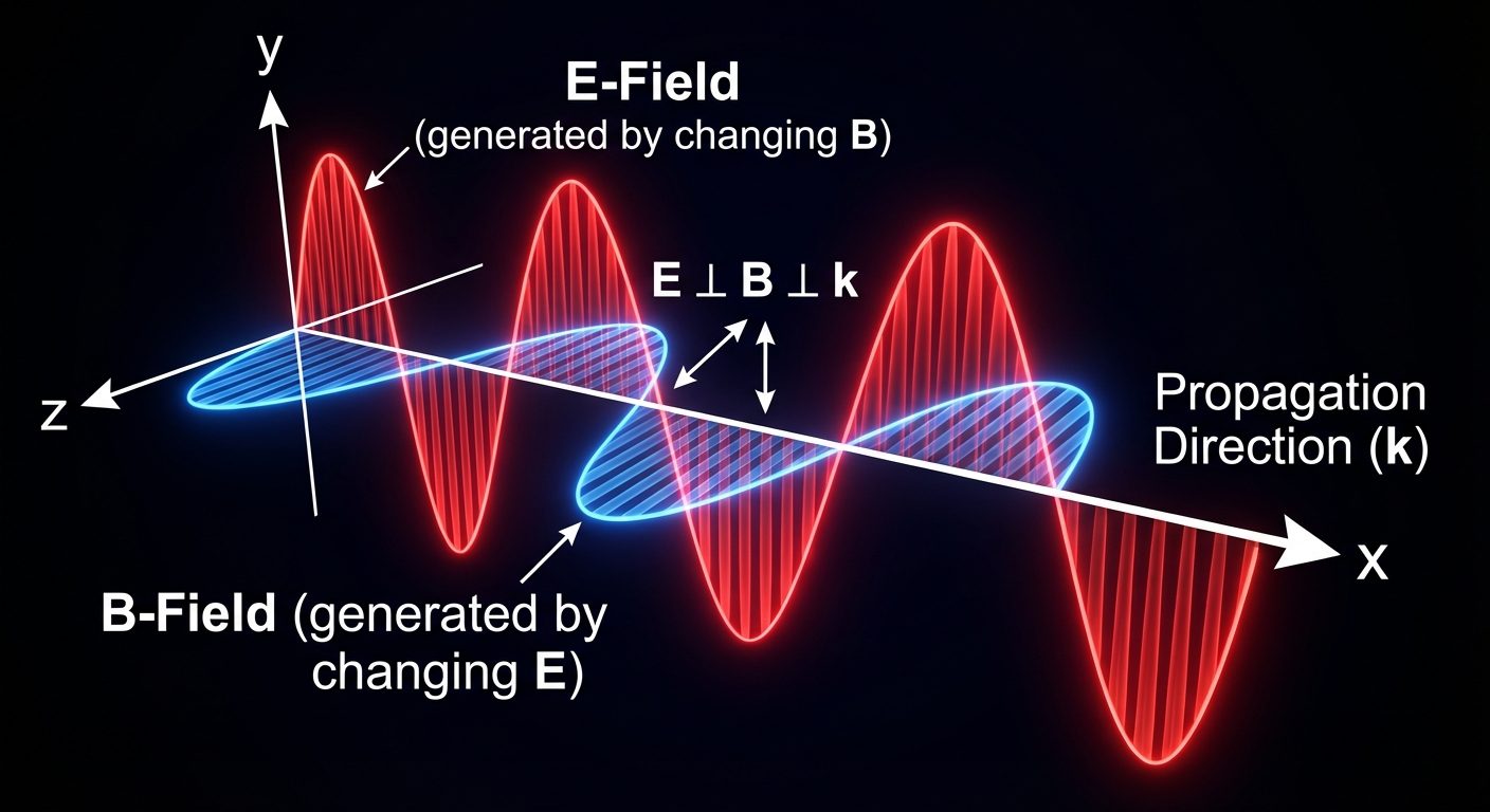
4. Ampere-Maxwell Law ( $\nabla \times \vec{H} = \vec{J} + \frac{\partial \vec{D}}{\partial t}$ )

Magnetic fields are produced by two sources:
1. Conduction Current ( $\vec{J}$ ): Moving electric charges (current in a wire).
2. Displacement Current ( $\frac{\partial \vec{D}}{\partial t}$ ): Time-varying electric fields.
This equation proves that changing electric fields produce magnetic fields, completing the symmetry necessary for the propagation of Electromagnetic Waves.

A conceptual 3D visualization of an Electromagnetic Wave propagating in space to illustrate the sign... — AI-generated image — may contain inaccuracies

Unit 2